Assessment and weekly assignments

• The assessment covering this material will be in January (exact date TBC).
• Each week on Tuesday at 2 pm:
  • Last week’s assignment is collected.
  • The next week’s assignment is released.

Using the assignments effectively

• Try to re-derive at least one equation from the notes each week.
• Implement small pieces of the algorithms yourself in Python/NumPy.
• Use built-in libraries (e.g. scikit-learn) to check your answers.
• Ask questions early if a step in a derivation doesn’t make sense.

NumPy recap

• numpy.ndarray = fast, vectorised multi-dimensional array.
• ML models almost always work with matrices of shape (n_samples, n_features).
• Linear models are naturally written as X @ w.
• We will use NumPy to implement parts of logistic regression ourselves.

Arrays vs Python lists

Python lists do repetition, NumPy arrays do maths:

import numpy as np

lst = [1, 2, 3]
print(lst * 2)      # [1, 2, 3, 1, 2, 3]

arr = np.array([1, 2, 3])
print(arr * 2)      # [2, 4, 6]

• Lists are general containers.
• NumPy arrays support fast, elementwise arithmetic - ideal for ML.

Shapes and matrix multiplication

import numpy as np

X = np.array([[1.0, 2.0],
              [3.0, 4.0],
              [5.0, 6.0]])   # shape (3, 2)

w = np.array([0.1, 0.2])     # shape (2,)

z = X @ w                    # shape (3,)
print(z)

• X: 3 samples, 2 features each.
• w: weights of a linear model.
• X @ w computes \(z^{(i)} = w^\top x^{(i)}\) for all rows at once.

Indexing and slicing

X = np.arange(12).reshape(3, 4)
# X =
# [[ 0  1  2  3]
#  [ 4  5  6  7]
#  [ 8  9 10 11]]

first_row  = X[0, :]
second_col = X[:, 1]
submatrix  = X[1:, 2:]

• X[i, :] = i-th row, all columns.
• X[:, j] = j-th column, all rows.
• X[a:b, c:d] = block of rows a..b-1, columns c..d-1.

Logistic regression and Loss functions

The problems we had with the perceptron were:

• only converged for linearly separable problems
• stopped in places that did not look like they would generalise well

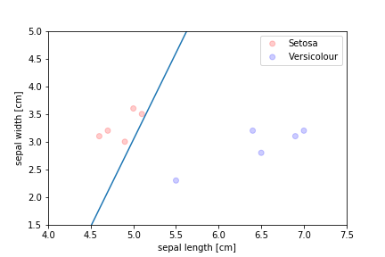
We need an algorithm that takes a more balanced approach:

• finds a "middle ground" decision boundary
• can make decisions even when the data is not separable
• ideally: gives us probabilities, not just hard labels

Probability vs. Odds

• Probability \(p\): “How often the event occurs.”
• Odds:
  \[ \frac{p}{1-p} \]
  “How often the event occurs compared to how often it doesn't.”

Why this definition?

Odds measure relative likelihood.

• \(p = 0.50 \Rightarrow\) odds = 1 (equally likely)
• \(p = 0.75 \Rightarrow\) odds = 3 (3× more likely)
• \(p = 0.20 \Rightarrow\) odds = 0.25 (1/4 as likely)

From probability to odds

• Binary classification: positive class \(y=1\), negative class \(y=0\).
• Let \(p = P(y=1 \mid x)\) be the probability of the positive class.
• The odds of the positive class are \[ r = \frac{p}{1-p}. \]
• \(r > 1\): positive class more likely; \(r < 1\): negative class more likely.

Why not just threshold a linear regression?

• Idea: fit a linear model with squared error and predict class 1 if \(\hat{y} > 0.5\).
• Problems:
  • Predictions can be < 0 or > 1 - not valid probabilities (y = mx + c).
  • Gradients can be small in exactly the regions where we care most.
• Logistic regression directly models \(P(y=1\mid x)\) with a proper probabilistic loss.

Log-odds (logit)

• Odds range from 0 to infinity
• Linear regression models output predictions from -infinity to infinity
• Define the log-odds (logit) as \[ z = \log r = \log \frac{p}{1-p}. \]
• \(z\) is unbounded: can be any real number.
• We model \(z\) with a linear function of the features: \[ z = w_0 + \sum_{j=1}^{D} w_j x_j. \]
• This is why it is still called a regression model.

From log-odds to probability

We can invert the relationship between \(p\) and \(z\):

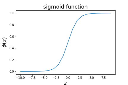
$$ p = \frac{1}{1 + e^{-z}} \equiv \phi(z). $$

• \(\phi(z)\) is the sigmoid function.
• For large positive \(z\), \(\phi(z) \approx 1\); for large negative \(z\), \(\phi(z) \approx 0\).
• The decision boundary at \(p = 0.5\) corresponds to \(z = 0\), i.e. \(w_0 + w^\top x = 0\) (a hyperplane).

Extreme scores don’t change much

• \(z = 10 \Rightarrow \phi(z) \approx 0.99995\)
• \(z = 100 \Rightarrow \phi(z) \approx 1 - 3.7\times10^{-44}\)
• \(z = 10000 \Rightarrow \phi(z) \approx 1\) to machine precision

Once \(z\) is very large or very negative:

• Predicted probability is essentially 0 or 1.
• Gradient \(\phi'(z)\) is ~0 ⇒ almost no learning signal.

This is why we care most about the “uncertain” region near \(z=0\).

Sigmoid

In ML sigmoids belong to a class of functions called "activation functions".

They introduce non-linearity in neural networks which will we cover later in the course.

Sigmoid function in NumPy

import numpy as np

def sigmoid(z):
    return 1.0 / (1.0 + np.exp(-z))

z = np.linspace(-6, 6, 13)
print(sigmoid(z))

• \(\phi(z) = \dfrac{1}{1+e^{-z}}\) applied elementwise.
• z can be a scalar, vector, or matrix.
• This is the link between linear scores and probabilities in logistic regression.

Vectorised logistic regression

def predict_proba(X, w, b):
    z = X @ w + b          # linear scores
    return sigmoid(z)      # probabilities in (0, 1)

def predict_class(X, w, b, threshold=0.5):
    p = predict_proba(X, w, b)
    return (p >= threshold).astype(int)

• Decision rule: predict class 1 if \(\hat{p} \ge 0.5\), else 0.
• Changing the threshold changes how "conservative" the classifier is.

Loss function with a two class model

How do we know whether our predictions are good?

If we have two classes, we call one the positive class ($c=1$) and the other the negative class ($c=0$). If the probability to belong to class 1

$$p(c=1) = p$$

we also have

$$ p(c=0)=1-p $$

The likelihood for a single measurement if the outcome is in the positive class is $p$ and if the outcome is in the negative class the likelihood is $1-p$. For a set of measurements with outcomes $y_i$ the likelihood is given by

$$ L = \prod\limits_{y_i=1} p \prod\limits_{y_i=0} (1-p) $$

So the negative log-likelihood is:

$$ NLL = - \sum\limits_{y_i=1} \log(p) - \sum\limits_{y_i=0} \log(1-p) $$

Given that $y=0$ or $y=1$ we can rewrite it as

$$ NLL = - \sum \left( y \log(p) + (1-y)\log(1-p) \right) $$

So if we have a model for the probability $\hat y = p(X)$ we can maximize the likelihood of the training data by optimizing

$$ J= - \sum_i y_i \log \left(\hat y\right) +(1-y_i)\log\left(1 - \hat y\right) $$

It is called the cross entropy.

Cross-entropy vs 0–1 loss

Why not just set the loss directly as 0 or 1?

• 0–1 loss:
  • 0 if prediction is correct, 1 if incorrect.
  • Exactly matches classification accuracy.
  • But non-differentiable and hard to optimise directly.
• Cross-entropy:
  • Smooth surrogate for 0–1 loss.
  • Gives useful gradients even for "almost wrong" examples.
  • Encourages calibrated probabilities, not just correct labels.

Logistic regression optimisation

• We choose the parameters \(w\) and \(b\) by minimising a loss function.
• The standard choice for logistic regression is the cross-entropy loss:

$$ J(w) = - \sum_i \left[ y^{(i)} \log \big(\phi(z^{(i)})\big) + (1-y^{(i)}) \log \big(1-\phi(z^{(i)})\big) \right], $$

• Only one of the log terms is "active" for each data point.
• If the model is confidently wrong, the loss becomes very large.

Cross-entropy vs squared error

• Squared error: \[ J_{\text{SE}} = \sum_i (y^{(i)} - \hat{y}^{(i)})^2. \]
• Cross-entropy: \[ J_{\text{CE}} = - \sum_i \big[ y^{(i)} \log \hat{y}^{(i)} + (1-y^{(i)})\log(1-\hat{y}^{(i)}) \big]. \]

For classification:

• Cross-entropy comes from a Bernoulli likelihood model.
• It focuses the gradient where it matters: misclassified or uncertain examples.
• Squared error is less well matched to 0/1 targets and can give weaker gradients near 0 or 1.

How do we minimize the cross entropy loss?

Gradient descent

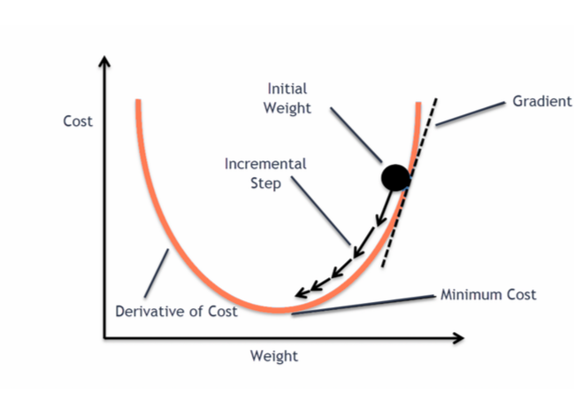
To optimise the parameters \(w\) we calculate the gradient of the loss function \(J\) and move in the opposite direction.

$$ w_j \rightarrow w_j -\eta \frac{\partial J}{\partial w_j} $$

\(\eta\) is the learning rate, it sets the speed at which the parameters are adapted.

It has to be set empirically.

Sigmoid saturation

$$ \phi(z) = \frac{1}{1+e^{-z}}, \qquad \phi'(z) = \phi(z)\bigl(1-\phi(z)\bigr). $$

Some values:

• \(z = -5 \Rightarrow \phi(z) \approx 0.007\)
• Thus \(\phi'(z) \approx 0.007\)
• \(z = 0 \Rightarrow \phi(z) = 0.5\)
• Thus \(\phi'(z) = 0.25\) (maximum slope)
• \(z = 5 \Rightarrow \phi(z) \approx 0.993\)
• Thus \(\phi'(z) \approx 0.007\)

For large \(|z|\) the sigmoid is almost flat: very small gradient.

Where does the model learn the most?

Imagine four examples with scores \(z\):

• A: z = -4
• B: z = -0.2
• C: z = 0.7
• D: z = 8

For which ones is the gradient \(\phi'(z) = \phi(z)(1-\phi(z))\) largest?

• B and C: \(z\) near 0 ⇒ \(\phi(z)\) around 0.5 ⇒ \(\phi'(z)\) large.
• A and D: saturated probabilities ⇒ tiny gradients.

Moral: examples the model is unsure about drive most of the learning.

How big a "step" should we take per gradient update?

Finding a suitable learning rate \(\eta\) is not always easy.

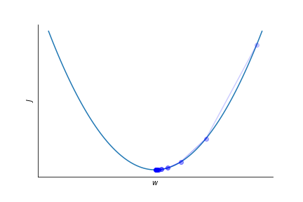
Finding a suitable learning rate \(\eta\) is not always easy.

A too small learning rate leads to slow convergence.

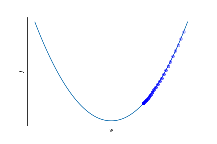
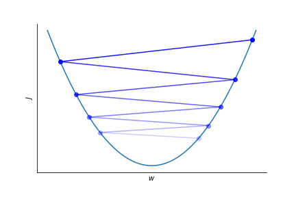
Too large learning rate might spoil convergence altogether!

Is there an issue with this method??

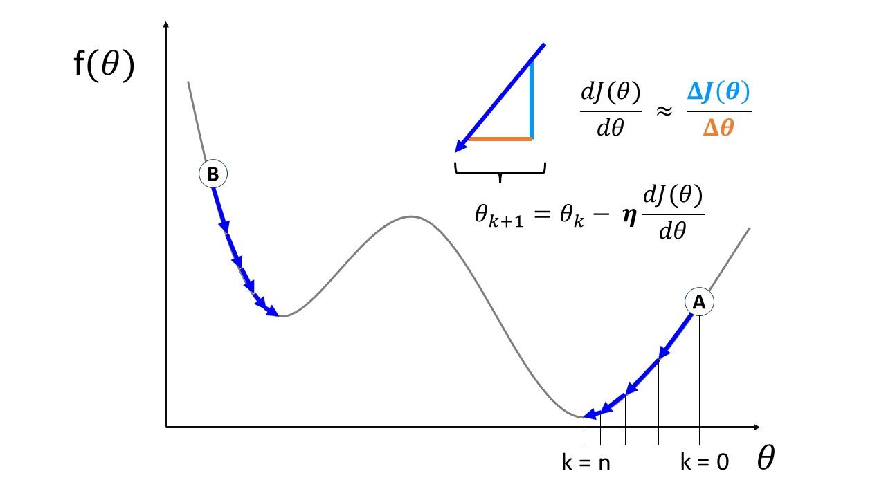
We're assuming no local minima

Derivative of the sigmoid

Recall \(\phi(z) = \dfrac{1}{1+e^{-z}}\). Differentiate with respect to \(z\):

$$ \frac{\mathrm{d} \phi}{\mathrm{d} z} = \phi(z)\,\big(1 - \phi(z)\big). $$

• This neat form is one reason the sigmoid is convenient.
• The derivative is largest near \(z=0\) and small in the saturated regions.

Gradient descent for logistic regression

Details of the derivative calculation:

$$ \frac{\partial \phi(z)}{\partial z} = \phi(z) (1-\phi(z)) $$

$$ \frac{\partial \phi}{\partial w_j} = \frac{\partial \phi(z)}{\partial z} \frac{\partial z}{\partial w_j} = \phi(z) (1-\phi(z)) x_j $$

$$ \begin{eqnarray} \frac{\partial J}{\partial w_j} &=& - \sum_i y_i \frac{1}{\phi(z_i)}\frac{\partial \phi}{\partial w_j} - (1-y_i)\frac{1}{1-\phi(z_i)}\frac{\partial \phi}{\partial w_j} \\ &=& - \sum_i y_i (1-\phi(z_i))x_j^{(i)} - (1-y_i)\phi(z_i)x_j^{(i)} \\ & = & - \sum_i (y_i - \phi(z_i)) x_j^{(i)}. \end{eqnarray} $$

where \(i\) runs over all data samples, \(1\leq i \leq n_d\) and \(j\) runs from 0 to \(n_f\).

Gradient of the logistic loss

For a single example \((x^{(i)}, y^{(i)})\) we have \(\hat{y}^{(i)} = \phi(z^{(i)})\) with \(z^{(i)} = w^\top x^{(i)}\).

Using the chain rule and the sigmoid derivative, one can show

$$ \frac{\partial J}{\partial w_j} = - \sum_i \big( y^{(i)} - \hat{y}^{(i)} \big) x_j^{(i)}. $$

• The error term \(y^{(i)} - \hat{y}^{(i)}\) is exactly "target minus prediction".
• Gradient descent update: \[ w_j \leftarrow w_j - \eta \frac{\partial J}{\partial w_j}. \]

Vectorised form of the gradient

• Stack features into a matrix \(X \in \mathbb{R}^{n \times D}\).
• Stack labels into a vector \(y \in \mathbb{R}^n\).
• Let \(\hat{y} = \phi(Xw)\) be the vector of predictions.

Then the gradient can be written compactly as

$$ \nabla_w J = - X^\top (y - \hat{y}). $$

• This matches the NumPy code X.T @ (y - y_hat).
• Shows clearly why vectorised operations are natural for ML.

Logistic regression example

two features relevant to the discrimination of benign and malignant tumors:

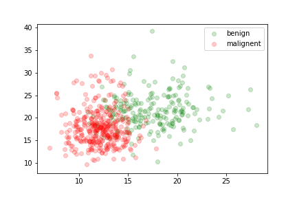
The data is not linearly separable.

We can train a sigmoid model to discriminate between the two types of tumors. It will assign the output class according to the value of

$$ z= w_0 + \sum_j w_j x_j = w_0 + (x_1,x_2) (\omega_1,\omega_2)^T $$

where \(\omega_0\), \(\omega_1\) and \(\omega_2\) are chosen to minimise the loss.

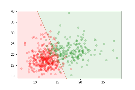
The delimitation is linear because the relationship between parameters and features in the model is linear.

The logistic regression gives us an estimate of the probability of an example to be in the first class

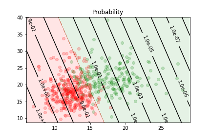
Checking with scikit-learn

from sklearn.linear_model import LogisticRegression

model = LogisticRegression()
model.fit(X_train, y_train)

print(model.coef_, model.intercept_)
print(model.predict_proba(X_test[:5]))
print(model.predict(X_test[:5]))

• LogisticRegression implements the same model with regularisation and smart optimisation.
• Useful as a reference to your implementation.

Regularisation

To reduce overfitting we often add an L2 penalty on the weights:

$$ J_{\text{reg}}(w) = J(w) + \lambda \|w\|_2^2. $$

• Encourages small weights (simpler models, smoother decision boundary).
• Helps especially when there are many correlated features.
• In scikit-learn’s LogisticRegression, the parameter C is roughly \(1/\lambda\).

Can think of this geometrically

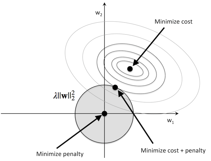
Geometric view of L2 regularisation

Regularised loss:

$$ J_{\text{reg}}(w) = J(w) + \lambda \|w\|_2^2. $$

• \(J(w)\): data fit (cross-entropy).
• \(\lambda \|w\|_2^2\): penalises large weights.
• Geometrically: choose a point where contours of \(J(w)\) meet a “circle” \(\|w\|_2\leq\) constant.

Result: smaller weights ⇒ smoother, less extreme decision boundary.

Normalising inputs (standardisation)

It is often useful to rescale each feature to have mean 0 and variance 1:

$$ x'_j = \frac{x_j - \mu_j}{\sigma_j}, $$

where \(\mu_j\) and \(\sigma_j\) are the mean and standard deviation of feature \(j\) on the training set.

• Helps keep \(z = w^\top x\) in a reasonable range.
• Avoids pushing the sigmoid into very flat (saturated) regions.
• Makes gradient descent behave better and converge faster.

Beyond binary classification: softmax regression

• For more than 2 classes, we generalise logistic regression with the softmax function.
• For class \(k\): \[ p_k = \frac{e^{z_k}}{\sum_{j} e^{z_j}}, \] where each \(z_k\) is linear in \(x\).
• Probabilities \((p_1,\dots,p_K)\) are non-negative and sum to 1.
• We train with a multi-class cross-entropy loss (very similar idea).

Softmax function

For class \(k\):

$$ p_k = \frac{e^{z_k}}{\sum_{j=1}^K e^{z_j}}. $$

• All \(p_k \ge 0\) and \(\sum_k p_k = 1\).
• Adding a constant to all \(z_k\) doesn’t change the probabilities.
• Large \(z_k\) ⇒ large \(p_k\), but still coupled to other classes.

Binary logistic regression is just the \(K=2\) special case.

Softmax cross-entropy

Encode the true class as a one-hot vector \(y\):

• \(y_k = 1\) for the true class, 0 otherwise.

The loss for one example is

$$ J = - \sum_{k=1}^K y_k \log p_k. $$

• Only the true class term is non-zero.
• If the model puts high probability on the true class ⇒ small loss.
• If it spreads mass on the wrong classes ⇒ large loss.

Softmax extends the classification to n

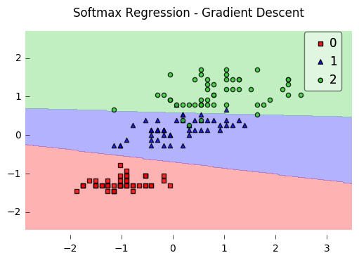
Softmax example

Three classes (e.g. A, B, C) and true class is A.

Two possible model outputs:

• Model 1: p = (0.7, 0.2, 0.1)
• Model 2: p = (0.4, 0.35, 0.25)

Which model has lower cross-entropy loss?

• Loss 1 = -log 0.7 = 0.155
• Loss 2 = -log 0.4 = 0.399

Model 1 wins!