Summative assignment
- Released 13th Jan 2026 at 2 pm and collected 2 pm 14th Jan 2026.
- Exam should take 3 hours but you have 24 hours to complete it.
- The server load is intense with everyone using it at the same time so the 24 hour window eases this.
- The exam does not take 24 hours to complete, aim for 3 hours.
- Entire script should run within 5 minutes.
- No collusion and No GenAI allowed.
Summative assignment Potential Topics
The assignment will cover topics you've already seen in the notebooks
- Data Cleaning and Feature Engineering.
- Logistic Regression
- Non-linear models
- Regularisation
- Bias–Variance Tradeoff
- Feed forward Neural Networks
- Dimensionality Reduction
- PCA and kNN (this week)
Summative assignment Non-Topics
This course covered extra ML techniques to aid your learning but will NOT be assessed
- CNNs
- Reinforcement Learning
- Transformers
- LTSM
- RNNs
- GANs (Generative Adversarial Networks)
- Self-Supervised Learning
- Support Vector Machines
The curse of dimensionality
One would think that the more features one has to describe samples in a dataset the better one would be able to perform a classification task. Unfortunately with the increase of the number of features comes the difficulty of fitting a multi-dimensional model.
This is generally referred to as the curse of dimensionality and we will see a few surprising effects that explain why more features can make life difficult.
How many points are in the center of the cube?
We can ask the question "In the hypercube $-1\leq x_i\leq 1$, how many points are no further apart to the center than 1?"
This is equivalent to asking what is the ratio of the unit "ball" to the volume of the smallest "cube" enclosing it.
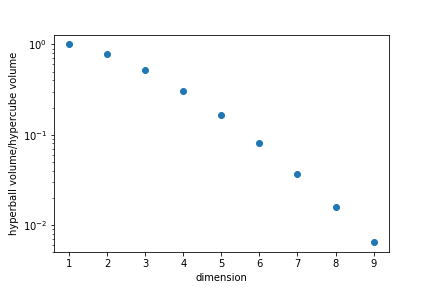
In high dimensions most points are in "corners" rather than in the "centre".
Average distance between two random points
Looking at the unit cube, we can calculate the average distance between any two points.
$$ d=\sqrt{\sum_i x_i^2} $$
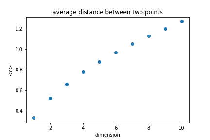
The average distance increases with the dimension.
We can also plot the distribution of distances:
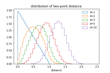
The likelihood of small distances drops as the dimension increases.
Proximity to edges
One interesting question to ask is how close to the edges points are. To quantify it we will calculate what is the thickness $t$ of the outer layer of the unit cube that contain half the points if the points are randomly distributed.
The volume inside is given by
$$ V_i = (1-2t)^d \qquad V_i=\frac12 \Rightarrow t = \frac{1-2^{-1/d}}{2}$$
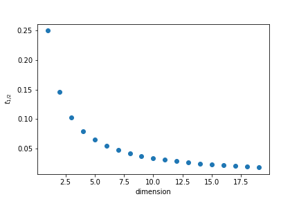
In 35 dimensions half of the points are in a outer layer 0.01 thin.
Principal component analysis
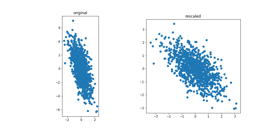
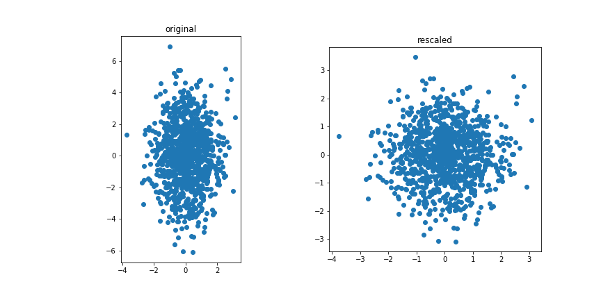
If we have many features, odds are that many are correlated. If there are strong relationships between features, we might not need all of them.
With principal component analysis we want to extract the most relevant/independant combination of features.
It is important to realise that PCA only looks at the features without looking at the labels, it is an example of unsupervised learning.
Correlated vs uncorrelated
Correlated features
Uncorrelated features:
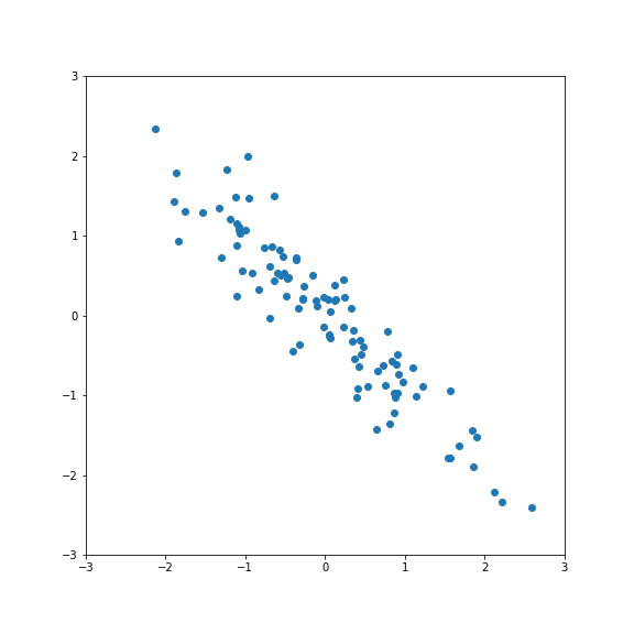
The idea for PCA is to project the (standardised) data on a subspace with fewer dimensions.
Standardization
Standarization involves transforming data so that each feature has a mean of 0 and a standard deviation of 1.
PCA is sensitive to the scale of the variables. Features with larger scales can dominate the principal components, skewing the results.
Illustrative Example:
- Consider a dataset with two features: height (in centimeters) and weight (in kilograms).
- Without standardization, height might dominate because its numerical values are larger.
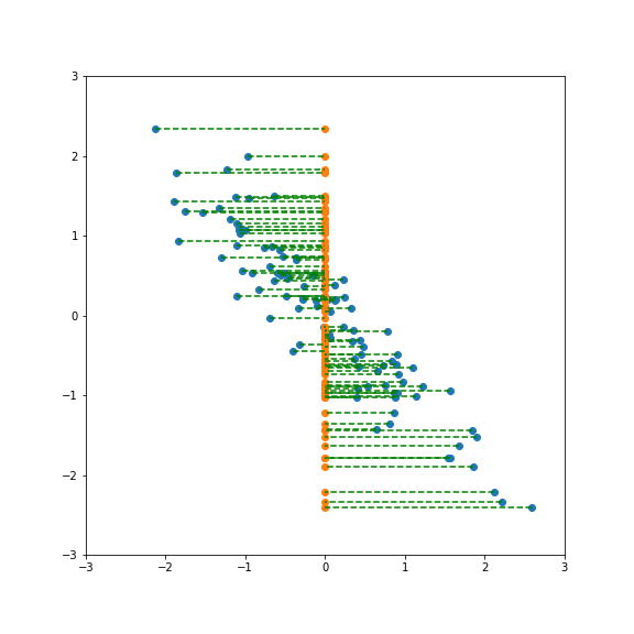
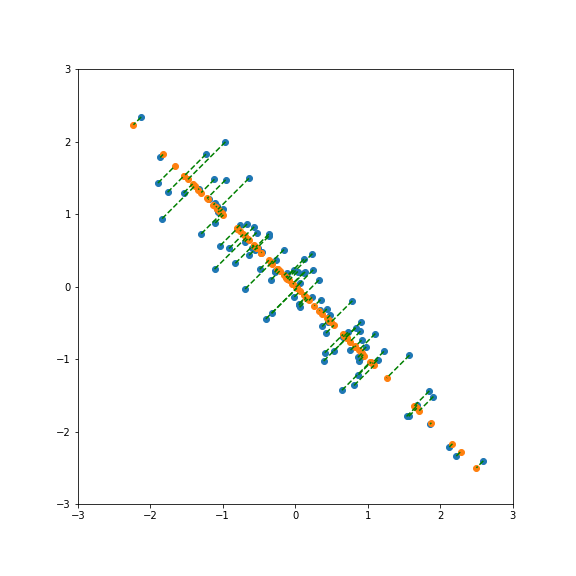
If we project onto the first component we get variance 1:
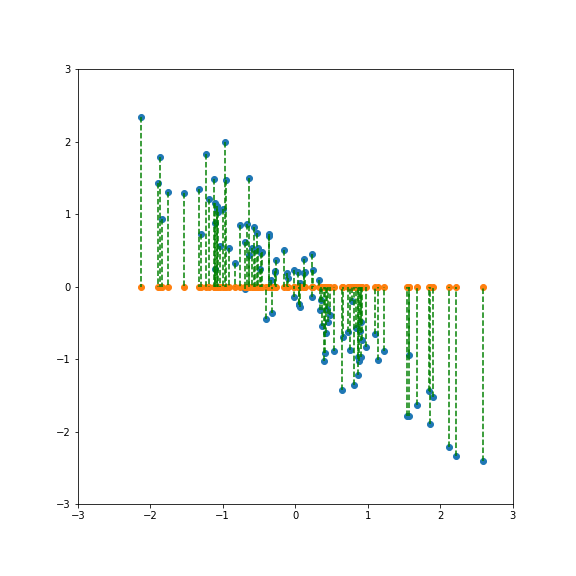
If we project onto the second component we also get variance 1:
But projecting onto a different direction gives a different variance, here larger than 1:
And here smaller than one:
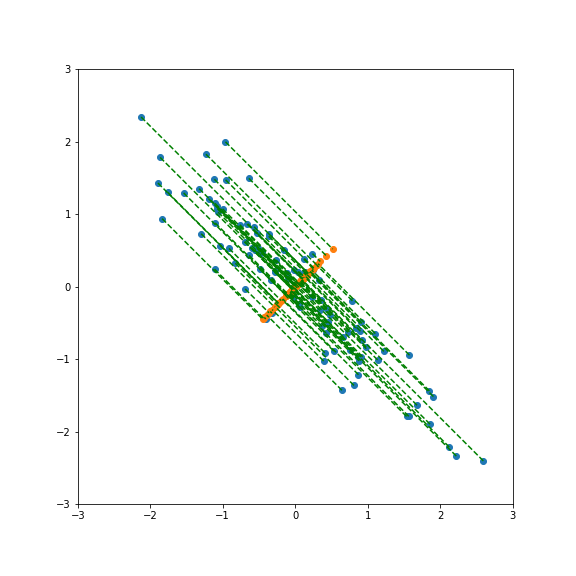
Performing PCA gives a new basis in feature space that include the direction of largest and smallest variance.
There is no guarantee that the most relevant features for a given classification tasks are going to have the largest variance.
If there is a strong linear relationship between features it will correspond to a component with a small variance, so dropping it will not lead to a large loss of variance but will reduce the dimensionality of the model.
Finding the principal components
The first step is to normalise and center the features.
$$ x_i \rightarrow a x_i +b $$such that
$$ \langle x_i\rangle = 0 \;,\qquad \langle x_i^2\rangle = 1$$The covariance matrix of the data is then given by
$$ \sigma = X^T X $$If $X$ is the $n_d\times n_f$ data matrix of the $n_d$ training samples with $n_f$ features. The covariance matrix is a $n_f\times n_f$ matrix.
Principal components as eigenvectors
After centering and normalising the data, PCA identifies the directions along which the dataset varies the most. These directions are obtained by diagonalising the covariance matrix
\[ \sigma = X^{T}X . \]The principal components are exactly the eigenvectors of this covariance matrix:
\[ \sigma\, v_j = \lambda_j\, v_j , \]where each eigenvector \(v_j\) defines a direction of maximal variance, and the corresponding eigenvalue \(\lambda_j\) equals the variance of the data along that direction.
Because the covariance matrix is symmetric, its eigenvectors form an orthonormal set. This means the principal components are pairwise orthogonal (i.e., independent), ensuring that the projected features are uncorrelated.
Explained variance
When we only consider the \(k\) principal axes of a dataset we will lose some of the variance of the dataset.
Assuming the eigenvalues are ordered in size we have
\[ \sigma_k \equiv \mathrm{Tr}(X_k^T X_k) = \sum_{j=1}^k \epsilon_j^2 \]\(\sigma_k\) is the variance our reduced dataset retained from the original; it is often referred to as the explained variance.
In practice, one often considers the explained variance ratio, defined as
\[ \frac{\sigma_k}{\sum_{j=1}^d \epsilon_j^2}, \]which measures the fraction of the total variance (the sum of all eigenvalues) captured by the first \(k\) principal components. This ratio is typically used to decide how many components are needed to retain a desired amount of information.
Example: 8x8 digits pictures
We consider a dataset of handwritten digits, compressed to an 8x8 image:
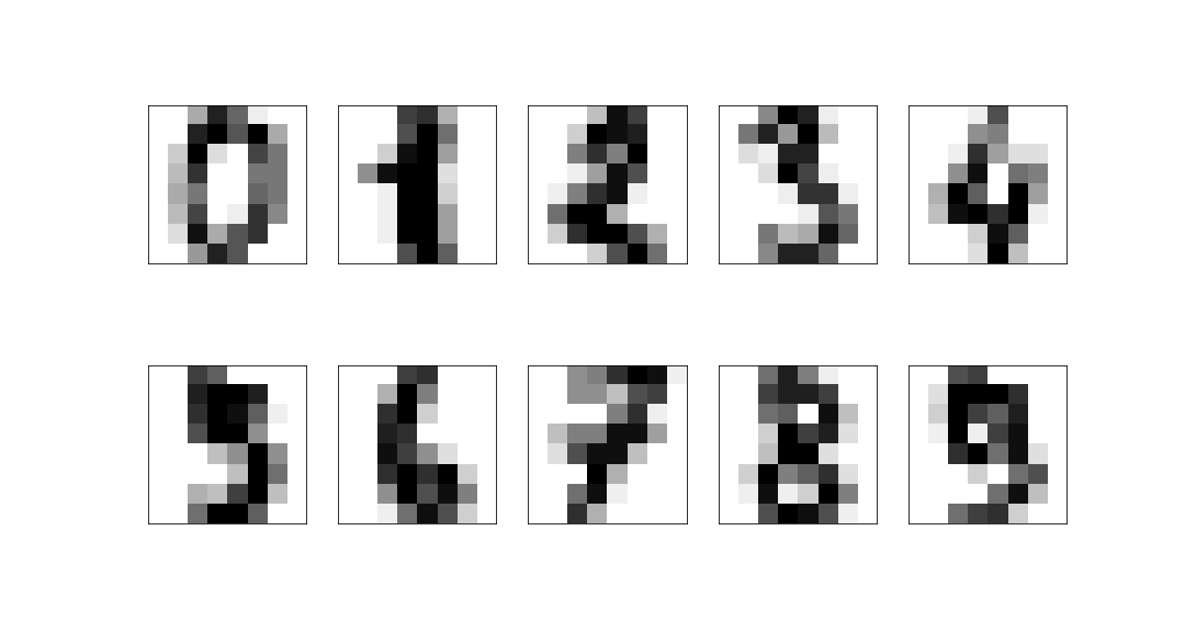
These have a 64-dimensional space but this is clearly far larger than the true dimension of the space:
- only a very limited subset of 8x8 pictures represent digits
- the corners are largely irrelevant hardly ever used
- digits are lines, so there is a large correlation between neighbouring pixels.
PCA should help us limit our features to things that are likely to be relevant.
Performing PCA we can see how many eigenvectors are needed to reproduce a given fraction of the dataset variance via a cumulative scree plot:
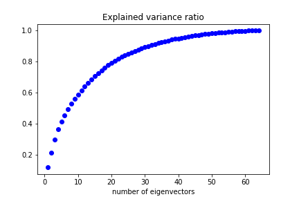
We can keep 50% of the dataset variance with less than 10 features.
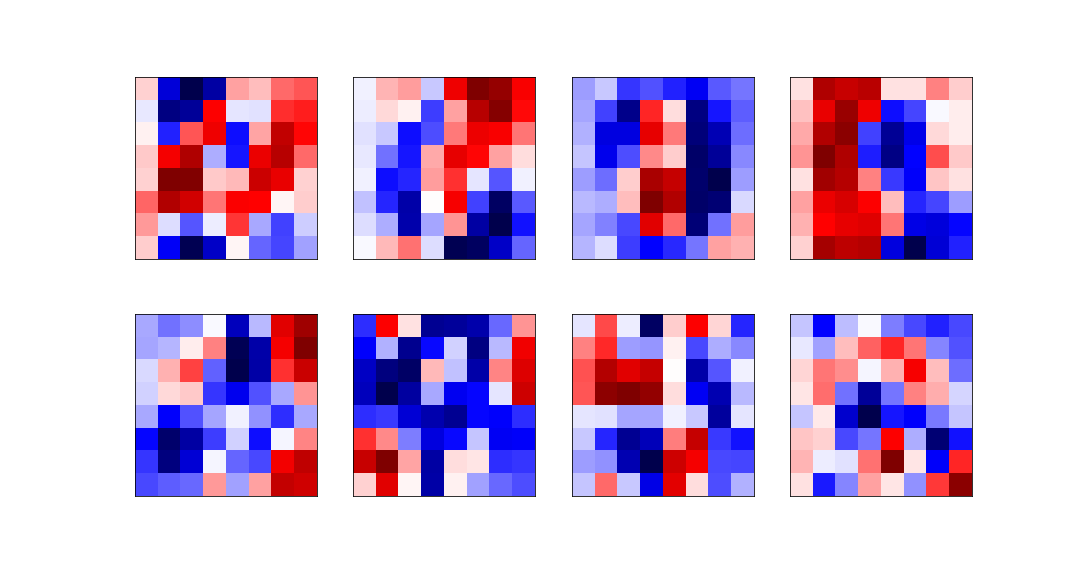
The eight most relevant eigenvectors are:
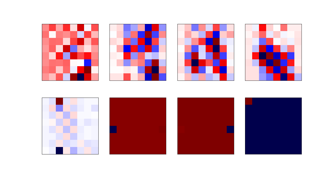
The least relevant eigenvectors are:
Data visualisation
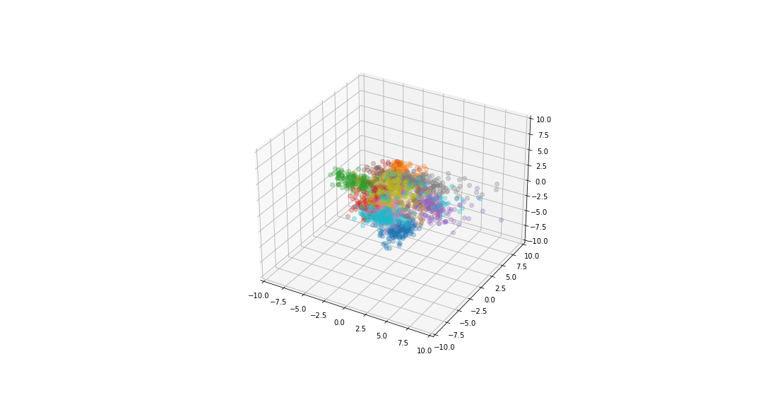
If we reduce the data to be 2-dimensional or 3-dimensional we can get a visualisation of the data.
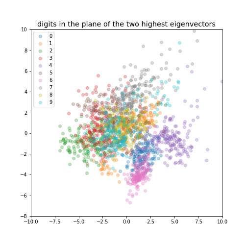
digits in the plane of the three highest eigenvectors
k-Neighbours
KNN
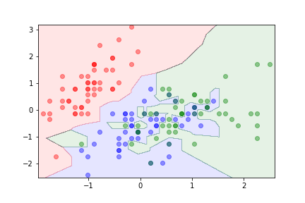
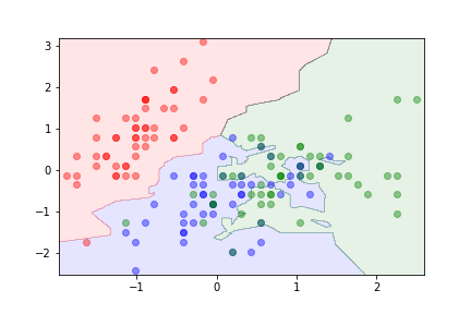
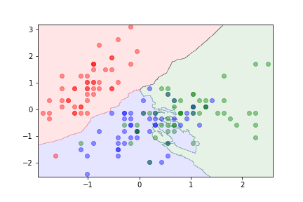
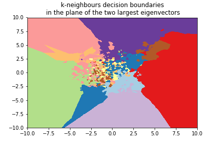
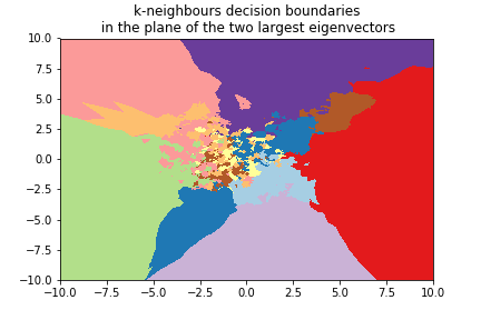
The parameter $k$ can be used to control overfitting.
- KNN is non-parametric (it makes no assumptions about the data's underlying distribution)
- KNN is lazy (it defers computation until the prediction phase).
- There's essentially no explicit training. KNN simply stores the training data.
- Basic procedure is compute distances, identify the 'k' closest data points, vote/average the class.
The kNN Algorithm
- Choose the number of neighbors, $k$.
- For a new sample point:
- Calculate the distance to all points in the dataset.
- Sort the points by distance.
- Pick the top $k$.
- Assign the most common class among the $k$ neighbors.
K-Nearest Neighbors (KNN)
The $k$-nearest neighbors method is an instance-based learning algorithm.
- It memorizes the training set.
- For a new data point, it finds the $k$ closest samples from the training set.
- Returns:
- Regression: The average of the target values of these $k$ neighbors.
- Classification: The class most common among the $k$ neighbors.
Intuition Behind KNN
Key Idea: Similar data points are likely to have similar target values.
- KNN uses the idea of proximity to predict the target variable.
- No explicit model is trained; all computations are deferred until prediction.
Advantages:
- Simple to understand and implement.
- Non-parametric: Makes no assumptions about data distribution.
Disadvantages:
- Computationally intensive with large datasets.
- Performance depends on the choice of $k$ and the distance metric.
Minkowski Distance
A generalization of both Euclidean and Manhattan distance:
$$d(p, q) = \left( \sum_{i=1}^n |q_i - p_i|^p \right)^{1/p}$$
- $p=1$: Manhattan
- $p=2$: Euclidean
Choosing k: The Goldilocks Problem
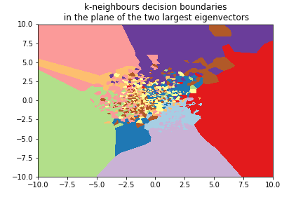
k = 1 (Too Small)
- The model is very sensitive to noise.
- Complex decision boundaries.
- High Variance (Overfitting).
Choosing k: The Goldilocks Problem
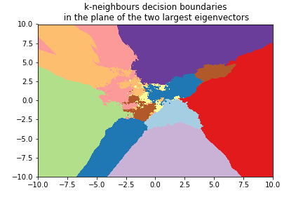
k = Large (Too Big)
- The model is too smooth.
- Captures the majority class, ignores local structure.
- High Bias (Underfitting).
Question
Q: If we have a dataset with $N$ points (50 red, 40 blue), and we set $k = N$, what happens?
A: The model will always predict the majority class (Red) for every single input.
The decision boundary disappears.
Voronoi Tessellation
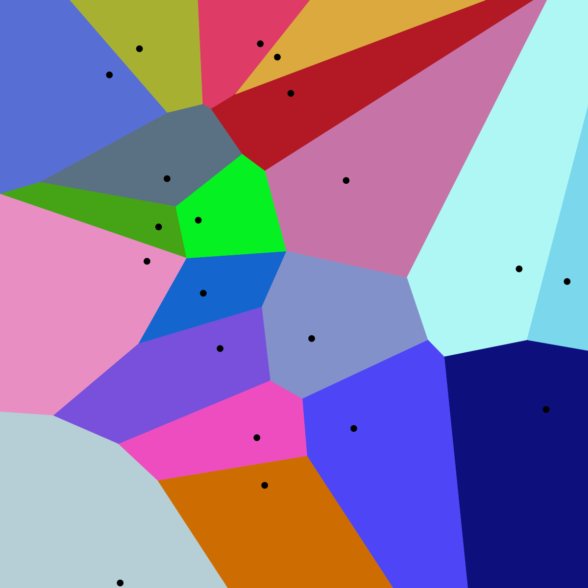
When $k=1$, kNN effectively divides the space into regions based on which point is closest.
These regions are called Voronoi Cells.
kNN and the Curse
Why did we learn these topics together?
The Problem with kNN in High Dimensions
kNN relies entirely on Distance.
As we saw in the "Curse of Dimensionality" section:
- In high dimensions, points become sparse.
- The ratio of distance to the nearest vs. farthest neighbor approaches 1.
In high dimensions, "nearest" becomes meaningless. All points are roughly equidistant.
Regularisation
The parameter $k$ can be used to control overfitting.
- With $k=1$ the algorithm is likely to overfit.
- Large values of $k$ can lead to underfitting.
Example
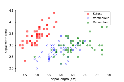
We can use the iris dataset:
k=1
k =3
k=10
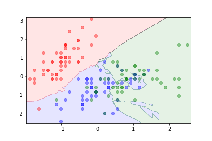
k=20
Digits example
We can use the 8x8 digits picture example after applying PCA to reduce it to 2 dimensions:
k=1
k=3
k=5
The Pipeline Solution
This creates a standard machine learning pipeline:
- Input: High-dimensional data.
- PCA: Reduce dimensions (e.g., from 100 to 10) to remove noise and curse effects.
- kNN: Run classification on the lower-dimensional data.
PCA rescues kNN from the curse.
Summary
- High dimensionality makes distance metrics unreliable (The Curse).
- PCA projects data to lower dimensions while preserving variance.
- kNN is a simple, effective classifier but struggles in high dimensions.
- Combining PCA + kNN is a powerful baseline strategy.