Non-linear models

Recap: What Linear Models Assume

Linear models operate under assumptions that often fail in real-world scenarios.

• The effect of each feature on the target is constant.
• Features combine additively - no multiplicative or complex interactions.
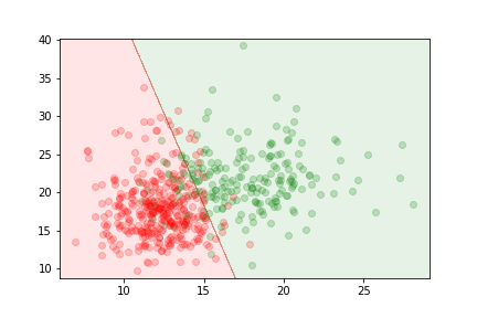
• Decision boundaries are hyperplanes.

These assumptions are elegant but restrictive.

When Linear Models DO Work Well

• Small datasets with clear trends.
• Domains where relationships are mostly monotonic.
• Engineering contexts with clean signals.

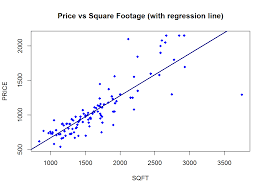
House price example: if all you use is square footage → price tends to increase linearly.

Why Non-linear Models?

Linear models make strong assumptions about the data:

• The relationship between features and the target is linear.
• Decision boundaries are straight lines.

Why Non-linear Models?

In many real-world problems, data is not linearly separable. Linear models, which use straight lines (or hyperplanes in higher dimensions) as decision boundaries, are insufficient for capturing complex patterns.

Non-linear models allow for more flexible decision boundaries, enabling us to model intricate relationships between features and target variables.

Real Data Rarely Behaves Linearly

In practice, relationships flatten, saturate, bend, or interact in strange ways.

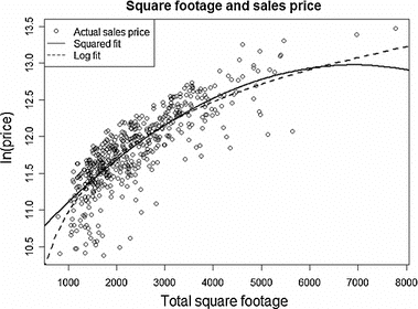
• House prices level off after a certain square footage (diminishing returns).
• Crime risk vs income is non-linear (sharp drop at a threshold).
• Health risk vs age increases exponentially, not linearly.

Feature Interactions are Everywhere

Example: predicting house price

• A 3-bedroom house in London vs in Newcastle has very different price effects.
• Square footage interacts with location.
• Bedrooms interact with number of bathrooms.

Linear models can’t express “the effect of X depends on Y”.

Example: House Price Non-linearity

Suppose we only use:

• square_footage
• num_bedrooms

The relationship between price and square footage may look like:

• Rapid increases for small homes
• Slower increases above ~2500 sqft

Example: House Price Non-linearity

Example: Salary Prediction

Salary vs experience is famously non-linear:

• Steep growth early career
• Plateau mid-career
• Sometimes drop in late career

Feature Engineering: The Fundamental Idea

Transform features → expose hidden structure → make simple models work on complex data.

Feature Scaling & Preprocessing

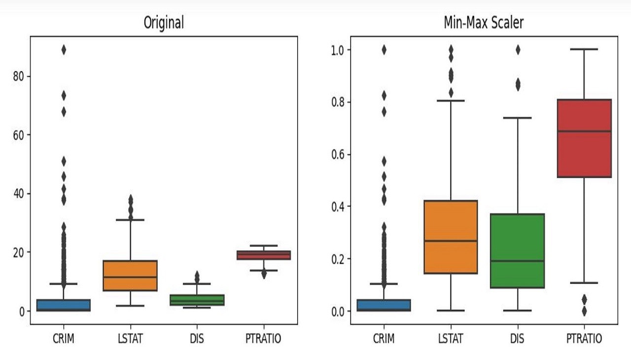
Even before creating new features:

• Standardizing (mean 0, variance 1)
• Normalizing to [0,1]
• Removing skew with log or sqrt

This is critical when feature magnitudes differ drastically.

Interaction Features

Example for house prices:

• location_score × bedrooms
• crime_rate × distance_to_city_cent

Interactions uncover effects that only appear when two features combine.

Ratio Features

These often encode intuitive human concepts.

• price_per_sqft = price / area
• bathroom_to_bedroom_ratio
• garden_size / total_plot_size

These ratios frequently outperform raw features.

Non-linear Transformations

Useful for:

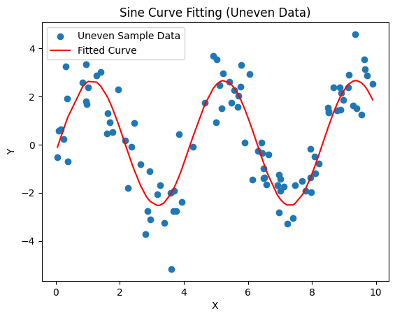
• Saturating processes (log)
• Explosive growth (exp)
• Seasonality (sin, cos)

Let's look at a separable problem that can't be linearly separated:

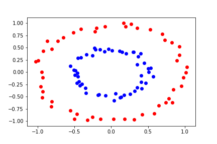
In this dataset, the two classes form concentric circles. No straight line can separate them perfectly.

Limitations of Linear Models

If we try to use a linear model and logistic regression, we do not get a good result.

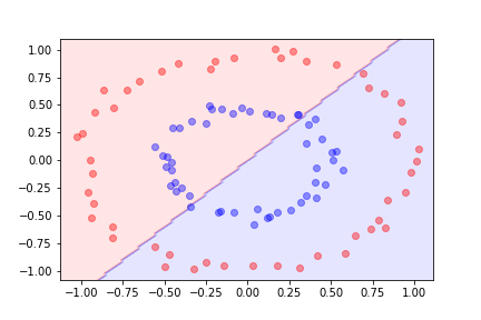
The linear model misclassifies many points because it cannot capture the circular pattern.

Transforming the Features

To separate the two sets linearly, we need to transform the data. Instead of using the original features x and y, we can use transformed features.

Let's use x² and y² as new features.

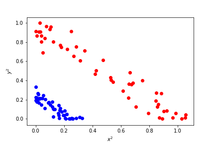
Now, in the transformed feature space, we can separate the data linearly!

Feature Engineering

Feature transformation is a part of feature engineering, where we create new features from existing ones to improve model performance.

Common transformations include:

• Polynomial features (e.g., x², xy, y²) – useful for capturing quadratic relationships.
• Interaction terms – combining features like age × income for socio-economic insights.
• Logarithmic and exponential transformations – handling skewed data such as income or population growth.
• Trigonometric functions?

These transformations can help models capture non-linear relationships.

Feature Engineering

Real-world example: Predicting House Prices

Feature engineering improves model predictions by creating meaningful transformations of raw data. For instance if you wanted to predict house prices and knew the sale price, square feet and number of bathrooms you can create new features:

• Price per Square Foot: Dividing the sale price by the property size gives a feature that often correlates strongly with market trends.
• Bedrooms per 1000 Sq. Ft.: Captures the "spaciousness" of the house, which may affect its attractiveness to buyers.

These features help models capture patterns that raw data alone might not reveal, improving performance and interpretability.

Adding Polynomial Features

In general, it is difficult to guess which transformation will help separate the data.

By adding polynomial features constructed from the existing ones, such as:

$$ (x, y) \rightarrow (x, y, x^2, y^2, xy) $$

we increase our separating power.

Effectively, we allow the straight lines in the linear model to become arbitrary curves if enough polynomial terms are added.

Using quadratic features in addition to the original ones, we can separate the datasets using logistic regression on the augmented feature space.

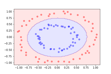
For more complicated boundaries, we can include higher-degree polynomial features.

Higher-Order Polynomial Features

Let's look at a different dataset:

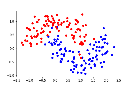
It is not linearly separable. Let's try second-order polynomial features.

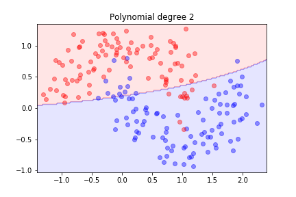
Second order is not sufficient; let's try degree 3...

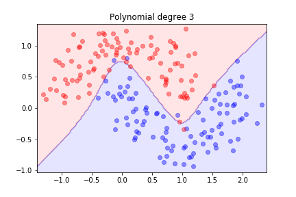
Better! What happens with higher degrees?

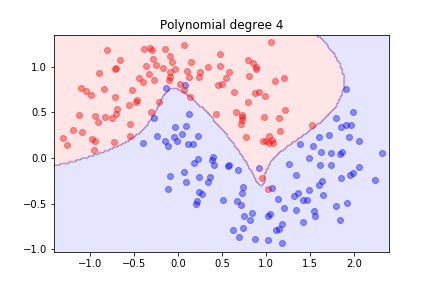
As we increase the degree, the model becomes more flexible and can fit the training data better.

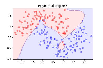
The model is trying hard to separate the data, but it might not generalize well.

Polynomial Features Explosion

Increasing degree quickly explodes feature count:

d features → polynomial degree k → binomial(d+k, k) features

Example: 10 features with degree 6 → ~5000 features!

Using polynomial features for this dataset:

We achieved a good separation on the training set, but we wondered how well the model might generalize.

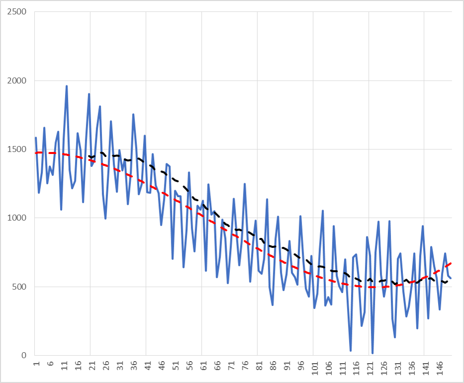
Noise vs Signal

The model learns “noise” when:

• data is limited
• model is too flexible
• features are too high-dimensional

>

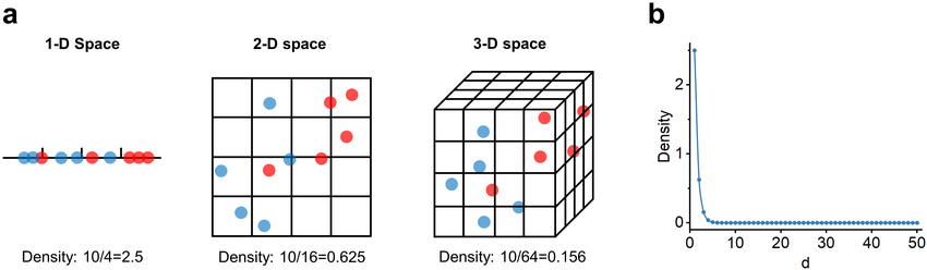
"Curse of Dimensionality"

As feature count increases:

• Data becomes sparse
• Distance metrics become unreliable
• Models need exponentially more data

>

Overfitting and Underfitting

Underfitting occurs when a model is too simple to capture the underlying pattern of the data.

Overfitting happens when a model is too complex and captures not only the underlying pattern but also the noise in the data.

Our goal is to find the right balance between underfitting and overfitting.

Overfitting and Regularisation

Overfitting occurs when a model learns the noise in the training data to the detriment of its performance on new data.

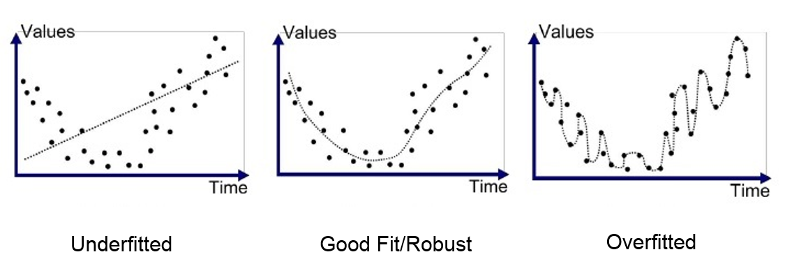
Why Overfitting Happens (Intuition)

Overfitting occurs because the model has too many ways to explain the data.

>

Regularisation: Adding "Friction"

Regularisation penalizes overly large coefficients.

It is like applying a smoothing force to stop the model bending too sharply.

L2 (Ridge) Intuition

Shrinks all coefficients toward zero.

Encourages simple boundaries.

all-regression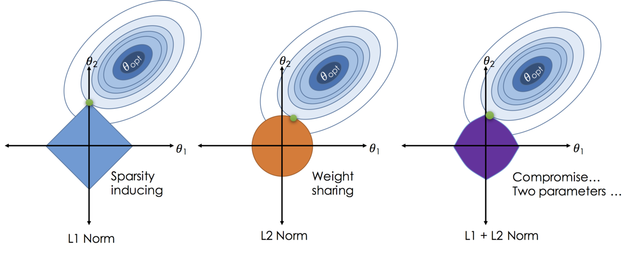

L1 (Lasso) Intuition

Pushes many coefficients *exactly* to zero.

This performs feature selection automatically.

Elastic Net

Combines L1 + L2.

Useful when many correlated features exist (common after polynomial expansion).

Evaluating Model Performance

To assess generalization, we need to evaluate the model on unseen data.

Common methods include:

• Splitting data into training and test sets
• Using cross-validation techniques
• Employing metrics like accuracy, precision, recall, F1-score

This helps us understand how the model performs on new, unseen data.

Testing the Model

The data was generated according to a fixed probability density. To evaluate the model's performance, we produce a separate, larger dataset that was not used during training. This ensures the model is tested on unseen examples, mimicking real-world scenarios.

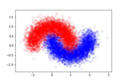
We will refer to this new dataset as the validation set, used specifically to assess the model's generalization capability.

As we increase the polynomial degree, the error on the training set decreases:

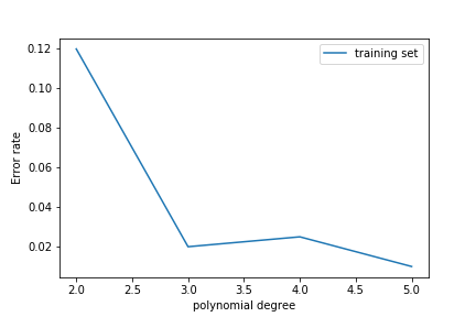
The error on the test set decreases at first but then increases again!

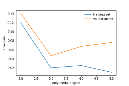
This is overfitting: the model learns the noise in the training set rather than the features of the underlying probability density.

Learning Curves

A learning curve shows how a model’s performance changes as it trains on more data.

Think of it like learning a new skill, such as cooking:

• At first: You make lots of mistakes (high error) because you’re inexperienced.
• With practice: You get better at following recipes (training error decreases).
• If you only practice one recipe: You struggle with new recipes (validation error stays high - overfitting).
• If you practice cooking different dishes: You improve overall, and mistakes on new recipes decrease (validation error drops).

Learning Curves - Formal

A learning curve shows how well a model performs as it is trained on more data.

It typically plots the error rate (e.g., misclassifications divided by total samples) or accuracy on two datasets:

• The training set, which the model learns from.
• The validation set, which tests how well the model generalizes to unseen data.

This visualization helps us understand whether the model is improving as it sees more data.

Interpreting Learning Curves

By comparing training and validation curves, we can diagnose model issues:

• High training error and high validation error: The model is underfitting and is too simple to capture patterns in the data.
• Low training error but high validation error: The model is overfitting, memorizing training data but failing to generalize.
• Converging training and validation errors: The model is learning well and generalizing appropriately.

Learning curves make it easier to identify and address these issues.

Learning Curves in House Price Example

If you train a model on:

• Only 50 houses → huge variance
• 5000 houses → stable generalization

Learning Curves in Medical Data

Models trained on small medical datasets almost always overfit:

• Skewed classes
• Subtle features

If the model is about right for the amount of training data we have, we get:

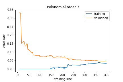
The training and validation sets converge to a similar error rate.

If the model is too simple, we get:

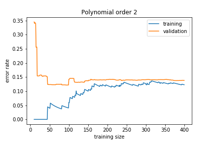
The training and validation errors converge but to a high value because the model is not general enough to capture the underlying complexity. This is called underfitting.

If the model is too complex, we get:

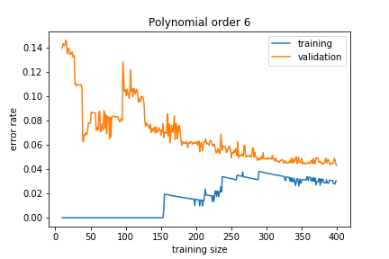
The training error is much smaller than the validation error. This means that the model is learning the noise in the training sample, and this does not generalize well. This is called overfitting.

Addressing Overfitting

To reduce overfitting, we can:

• Add more training data: Helps the model generalize better.
• Reduce model complexity: Simplify the model to prevent it from capturing noise.
• Use regularization: Penalize large coefficients in the model.
• Feature selection: Remove irrelevant or redundant features.
• Cross-validation: Ensure the model performs well on unseen data.

These strategies help improve the model's ability to generalize.

Adding more training data reduces the overfitting:

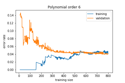
As we gather more data, the validation error decreases, and the model generalizes better.

Cross-Validation

Cross-validation is a technique for assessing how the results of a statistical analysis will generalize to an independent dataset.

K-Fold Cross-Validation:

• Divide the dataset into K equal subsets (folds).
• Train the model on K-1 folds and validate on the remaining fold.
• Repeat this process K times, each time with a different validation fold.
• Average the performance over the folds.

This provides a more robust estimate of model performance.

Common Mistakes in Non-Linear Models

• Using too many polynomial features with too little data.
• Not standardizing before polynomial expansion.
• Misinterpreting training accuracy as real accuracy.
• Forgetting cross-validation.

Practical Tip: Keep It Simple First

Before using polynomial features:

• Plot the data
• Fit a linear baseline
• Check for obvious structure in residuals

Often the baseline gives most of the performance.

How to Select Polynomial Degree

• Plot training + validation curves.
• Use cross-validation.
• Try degrees systematically.
• Use regularization for high degrees.

When NOT to Use Polynomial Features

• High-dimensional data (curse of dimensionality).
• Large datasets where non-linear models (e.g., trees) work better.
• When interactions are arbitrary or unknown.

Better Alternatives to Polynomial Features

• Decision trees / random forests
• Gradient boosting
• Neural networks
• Kernel SVMs

Conclusion

Non-linear models and feature transformations are powerful tools for handling complex datasets.

However, we must be cautious of overfitting and underfitting. Using techniques like regularization, cross-validation, and analyzing learning curves can help us build models that generalize well.

Understanding these concepts is crucial for effective machine learning.