Machine learning
A part of Core Ia: Introduction To Machine Learning And Statistics
Second half of Core Ia: Introduction To Machine Learning And Statistics.
Same procedure as part 1 with lectures and workshops on Tuesday and Friday. There are four notebooks but eight lectures.
Course website: https://miscada-ml-2526.notes.dmaitre.phyip3.dur.ac.uk/
Notebook server: https://miscada-ml-2526.notebooks.danielmaitre.phyip3.dur.ac.uk/

I'm Will Yeadon and will be organising this portion of the course
Can contact me via email will.yeadon@durham.ac.uk
Office is PH304 in Rochester Building
Course Content
- Week 6: Introduction to machine learning, Perceptron, Logistic regression, Loss functions
- Week 7: ROC curves, Support vector machines, Non-linear models, Learning curves, Regularisation
- Week 8: Variance-Bias trade-off, Neural networks
- Week 9: Dimensionality reduction, Principal component analysis, Unsupervised learning, K-neighbours, ML in python: sklearn and pandas
Contents
- Broad introduction to machine learning topics.
- Perceptron.
What is Machine learning?
What is Machine learning?

What is Machine learning?
Machine Learning
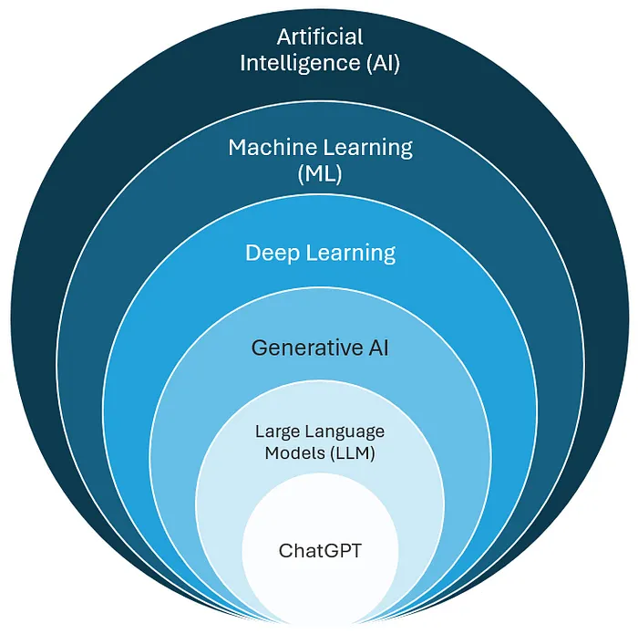
Machine Learning is a subset of artificial intelligence that focuses on enabling computers to learn from data and improve their performance over time without being explicitly programmed.
- Allows computers to identify patterns and make decisions with minimal human intervention.
- Utilized in various applications such as recommendation systems, speech recognition, and autonomous vehicles.
- Empowers organizations to make data-driven decisions.
Careers in Machine Learning
- Most ML careers focus on applying and deploying existing algorithms — building data pipelines, training models, and integrating them into products.
- Only a small fraction of roles involve inventing new algorithms (e.g. research labs, PhDs).
- Industry demand remains strong and growing across sectors — from finance and healthcare to logistics and creative industries.
- Key growth areas include MLOps (infrastructure and deployment), ML engineering (model training and serving), and data science (applied analysis).
- Generative AI has expanded opportunities — especially in model integration, evaluation, and retrieval‑augmented generation systems.
In short: a career in ML today means turning learning algorithms into reliable, scalable tools — not just developing new maths.
Machine learning algorithms can be classified according to:
- The type of problems they solve.
- The model they use.
- The way they learn.
- The type of data they process.
- The amount of human supervision involved.
Types of Problems
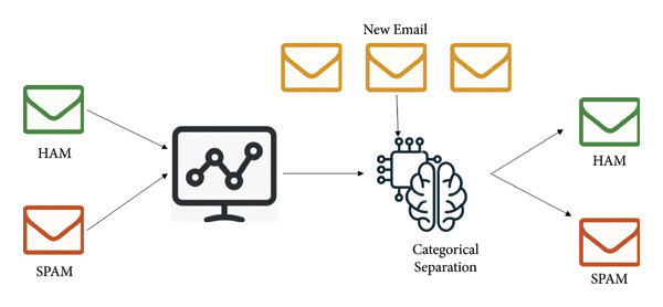
- Classification
- Output of the model is a discrete set of categories.
- Examples:
- Spam detection.
- Positive/negative COVID test.
- Image recognition (identifying objects in images).
- Sentiment analysis (classifying text as positive, negative, or neutral).
- Fraud detection in financial transactions.
Classification
Types of Problems
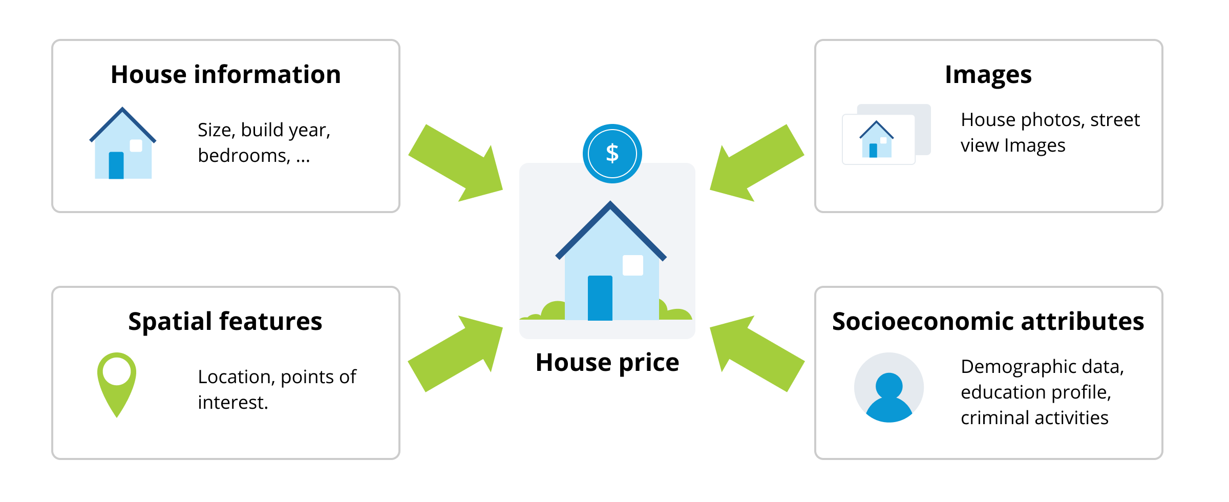
- Regression
- Output of the model is a continuous variable.
- Examples:
- Value of stock.
- Country GDP.
- Predicting housing prices.
- Forecasting weather temperatures.
- Estimating the lifetime of a machine component.
Regression
Types of Problems
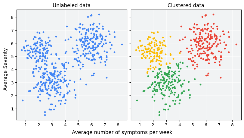
- Clustering
- Group data points into clusters based on similarity.
- Examples:
- Customer segmentation in marketing.
- Image Segmentation Tumor Detection (grouping pixels with similar properties like color and texture).
- Grouping genes with similar expression patterns.
- Community detection in social networks.
Clustering
Types of Problems
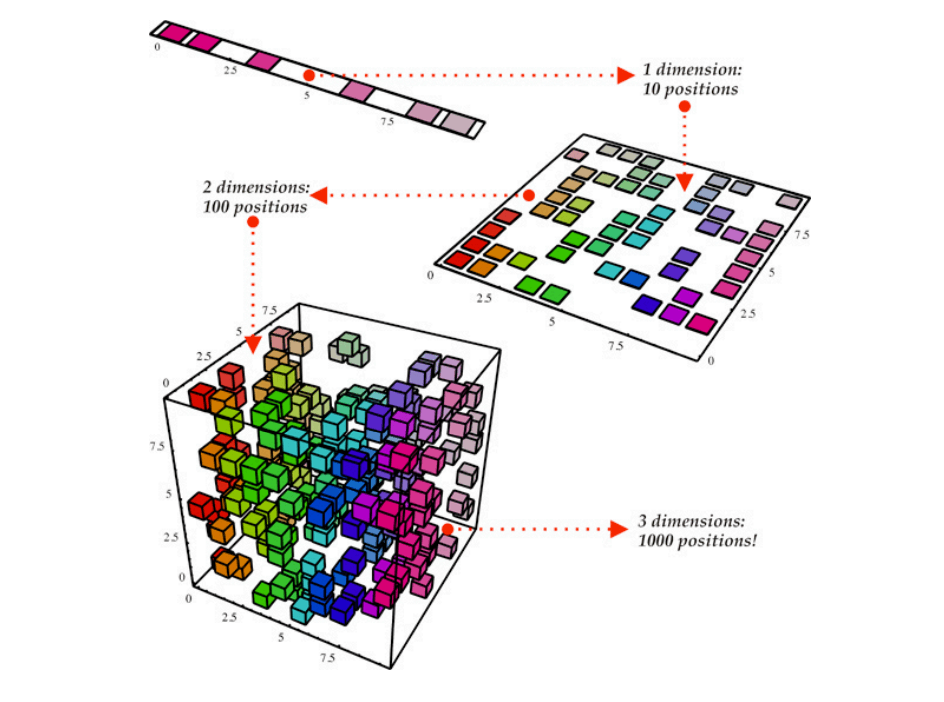
- Dimensionality Reduction
- Reduce the number of features while retaining important information.
- Examples:
- Principal Component Analysis (PCA).
- Reducing redundant variables (e.g., height and weight combined into BMI).
- Removing irrelevant features (e.g., door color when predicting house price).
- Combining correlated features into a single representative variable.
- Eliminating noise or low-variance features to improve model performance.
Dimensionality Reduction
 >
>
Types of Problems
The boundary between the two types can be blurred:
- When the categories have an ordering, we can use regression and bin the result into categories:
- A*, A, B, C, etc., grades.
- Number of stars for a review.
- Energy rating of a building.
- Credit score ratings.
- For classification, we can fit a function for the probability of belonging to one class:
- Logistic regression outputs probabilities between 0 and 1.
- Softmax function used in multi-class classification.
Some problems can be approached using either classification or regression techniques, depending on the desired outcome.
Types of Learning
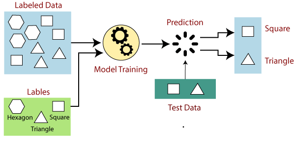
- Supervised Learning
- We have a training set with labeled examples.
- The algorithm learns a mapping from inputs to outputs.
- Examples:
- Detecting fraudulent credit card transactions.
- Predicting whether a patient has a disease from medical test results.
- Recognizing objects in images (e.g., cats vs. dogs).
- Forecasting tomorrow’s temperature from weather data.
Supervised Learning
Types of Learning
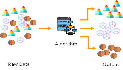
- Unsupervised Learning
- No labeled examples.
- The model has to find patterns or features.
- Can be used as a first step before supervised learning.
- Examples:
- Grouping news articles by topic without prior labels.
- Detecting anomalies in network traffic or sensor data.
- Discovering latent themes in large text corpora.
- Segmenting images into regions with similar color or texture.
Unsupervised Learning
Types of Learning
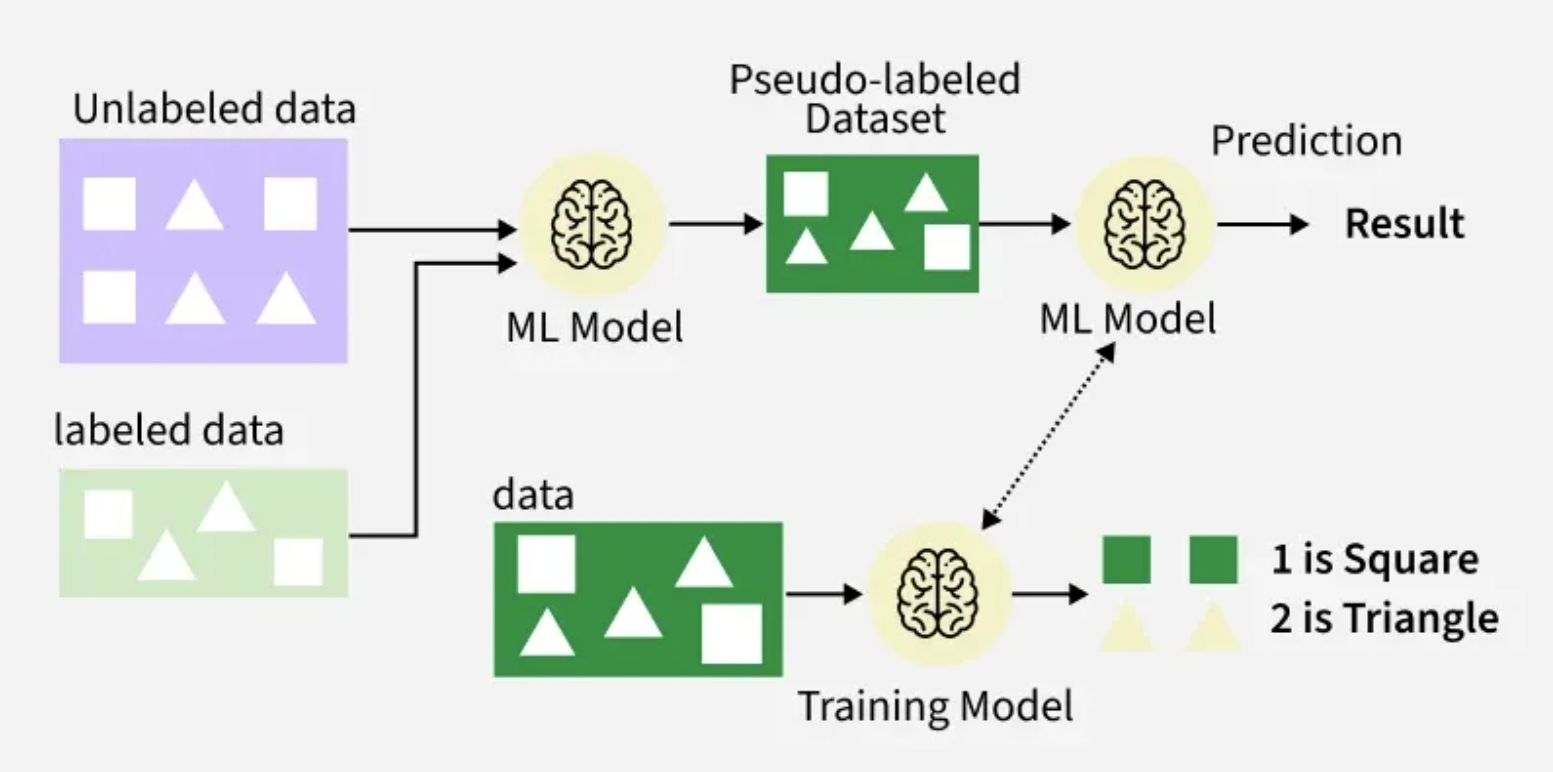
- Semi-supervised Learning
- Uses both labeled and unlabeled data.
- Helps when labeled data is scarce or expensive to obtain.
- Examples:
- Web content classification with limited labeled pages.
- Identifying sentiment in reviews when only a few are labeled.
- Training a medical image classifier using a few labeled scans and many unlabeled ones.
- Speech recognition trained on hours of unlabeled audio and a small set of transcribed samples.
Semi-supervised Learning
Reinforcement Learning
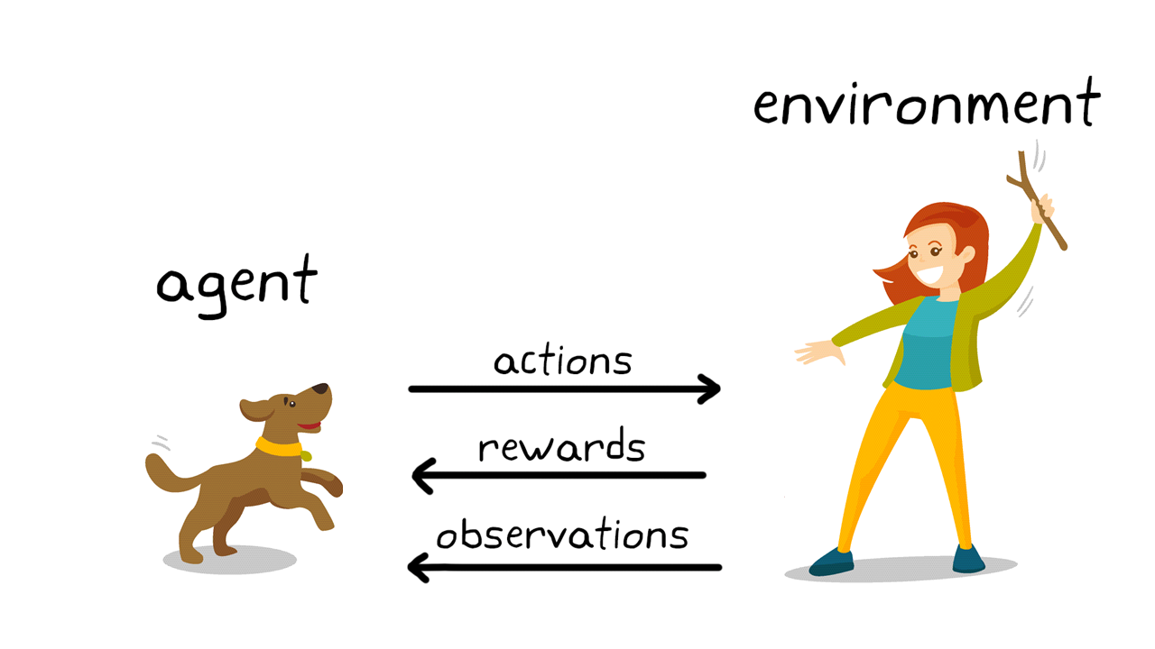
- Learning through trial and error.
- The model (agent) interacts with an environment.
- Receives rewards or penalties for its actions.
- Goal: Learn a policy that maximizes long-term (cumulative) reward.
How it Works
- At each step:
- The agent observes the state of the environment.
- It chooses an action.
- The environment provides a reward and a new state.
- The agent updates its policy based on experience.
- Repeat until the agent learns which actions yield the best outcomes.
Examples of Reinforcement Learning
- Game-playing AI (e.g., AlphaGo, chess, or Atari agents).
- Robotics — learning to walk, grasp, or balance.
- Autonomous driving — navigating and avoiding obstacles.
- Personalized recommendations — optimizing for engagement over time.
- Industrial control — adjusting manufacturing parameters dynamically.
Reinforcement Learning
Learning Modes
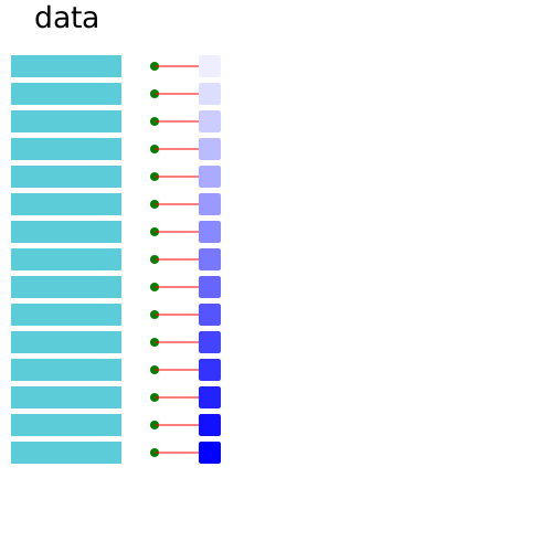
- Batch Learning
- The entire training set is used for each iteration of the model optimization.
- Requires significant memory and computational resources.
- Online Learning
- The model is updated for each new training example.
- Suitable for data that arrives in a stream or is too large to process all at once.
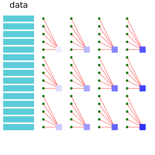
- Mini-batch Learning
- The model is optimized for subsets of the training set.
- Balances between batch and online learning.
- Improves computational efficiency and convergence stability.
Choosing the right learning mode depends on the dataset size and computational resources.
Batch Learning
The entire training set is used for each iteration of the model optimization.
Advantages:
- Stable convergence as it considers all data at once.
- Suitable for smaller datasets.
Disadvantages:
- Not scalable for very large datasets.
- High memory usage.
Online Learning
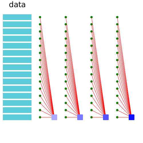
The model is updated incrementally as each new training example arrives.
Advantages:
- Can adapt to new data and changing environments.
- Suitable for real-time systems.
Disadvantages:
- May have less stable convergence.
- Requires careful tuning of learning rate.
Mini-batch
The model is optimized using small subsets (batches) of the training set.
Advantages:
- Reduces memory usage compared to batch learning.
- More computationally efficient than online learning.
- Smoother convergence than pure online learning.
Disadvantages:
- Requires choosing an appropriate batch size.
- May still be challenging with extremely large datasets.
Instance-based vs Model-based
- Instance-based
- Uses specific examples from the training data to make predictions.
- Relies on a similarity measure to compare new data to training data.
- Also known as "lazy learning" because it delays processing until a query is received.
- Model-based
- Abstracts from the training data to build a model that can make predictions.
- The data fixes the parameters of the model during training.
- Also known as "eager learning" because it builds the model before receiving queries.
The choice between instance-based and model-based methods depends on the problem at hand.
Example: Predicting final grade \( g_4 \) of a student given their 1st, 2nd, and 3rd-year results \( g_1 \), \( g_2 \), and \( g_3 \).
- Instance-based:
- Look at historical results and find the student(s) with the closest marks to the current student.
- Use the final grades of those past students as the prediction for the new student.
- Could average the final grades of the nearest neighbors.
- Model-based:
- Hypothesize a linear dependency: $$ g_4 = c_1 g_1 + c_2 g_2 + c_3 g_3 $$
- Fit the coefficients \( c_1 \), \( c_2 \), \( c_3 \) to historical data.
- Use the model to predict the new student's final grade.
This illustrates the fundamental difference in approach between the two methods.
Examples of Model-based Algorithms
- Linear Models
- Perceptron.
- Linear Regression.
- Logistic Regression.
- Support Vector Machine (SVM) with linear kernel.
- Non-linear Models
- Polynomial Regression.
- Decision Trees.
- Neural Networks.
- Random Forests.
- Support Vector Machine with non-linear kernels.
- Probabilistic Models
- Naive Bayes Classifier.
- Hidden Markov Models.
Model-based algorithms are powerful for capturing underlying patterns in data.
Examples of Instance-based Algorithms
- \( k \)-Nearest Neighbors (k-NN)
- Support Vector Machine (SVM) with Radial Basis Function (RBF) kernel
- Locally Weighted Learning
- Case-based Reasoning
- Kernel Regression
Instance-based methods are simple and effective for certain types of problems.
Perceptron
What is the perceptron?
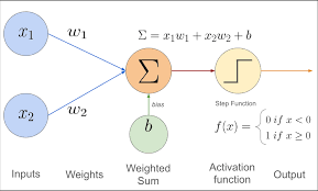
- Binary linear classifier: outputs +1 or −1 from a weighted sum of inputs and a threshold.
- Unit model: sign(w·x + b).
- Learning rule: iteratively tweaks weights when it makes a mistake.
History: Threshold neurons were formalised by McCulloch & Pitts (1943); the online learning algorithm was introduced by Frank Rosenblatt (1957–58).
Perceptron
Classification set‑up
We have training examples \((x^{(i)}, y^{(i)})\) with labels \(y^{(i)} \in \{+1,-1\}\).
Features: \(x^{(i)} = (x^{(i)}_1,\dots,x^{(i)}_{n_f})\in\mathbb{R}^{n_f}\).
Labels: \(y^{(i)}\in\{\pm 1\}\).
Model and decision rule
Score (affine):
\[ z(x; w,b) = w^\top x + b \]
Prediction (hard threshold):
\[ \hat y = \phi(z) = \operatorname{sign}(z) \in \{+1,-1\}. \]
Bias trick: augment \(\tilde x = (1, x_1,\dots,x_{n_f})\), \(\tilde w = (b, w_1,\dots,w_{n_f})\) so that \(z=\tilde w^\top \tilde x\).
Geometry
The set \(\{x : w^\top x + b = 0\}\) is a hyperplane (a line in 2D). It splits space into two half-spaces:
- \(w^\top x + b > 0\Rightarrow \hat y=+1\)
- \(w^\top x + b < 0\Rightarrow \hat y=-1\)
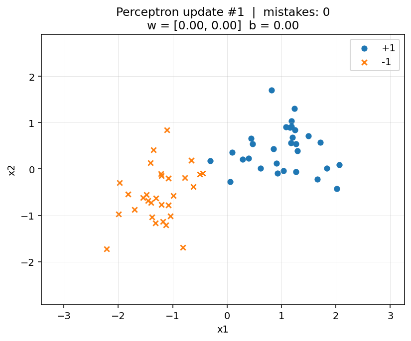
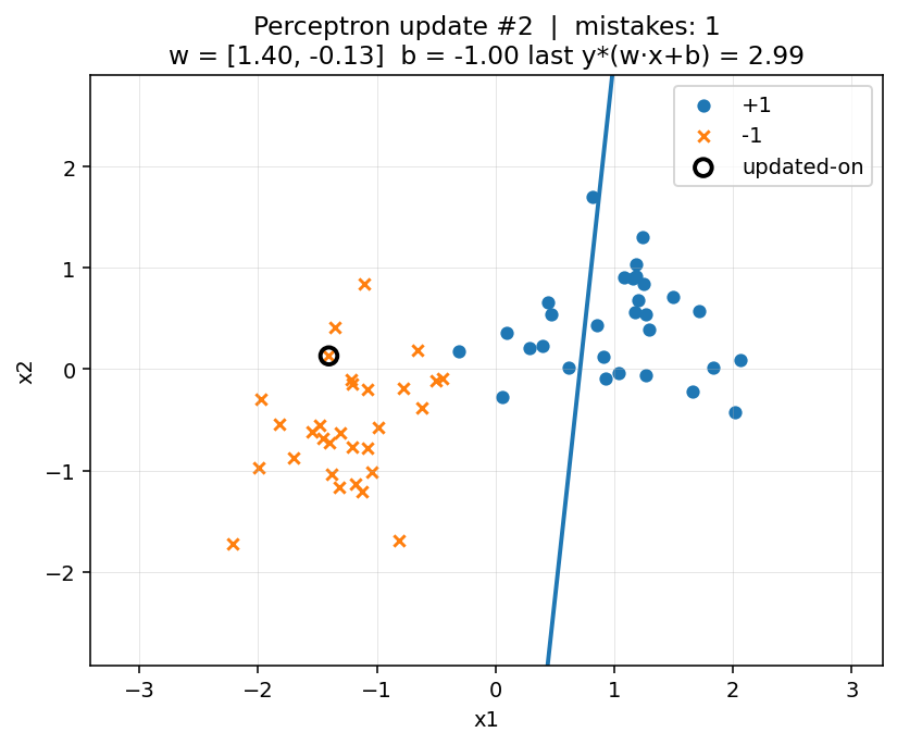
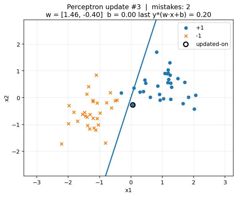
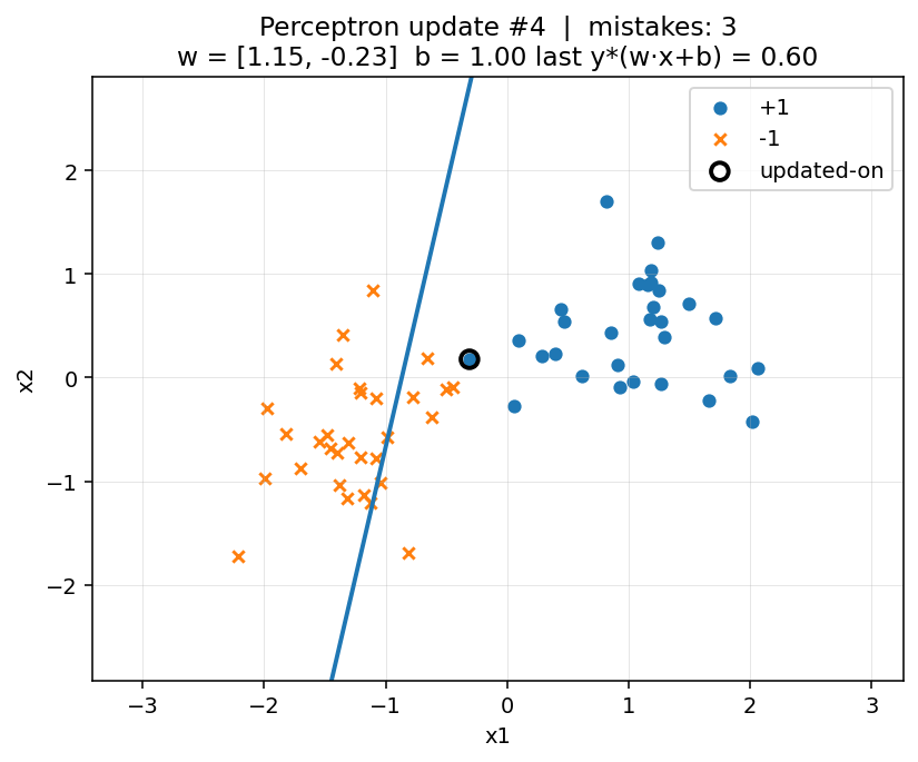
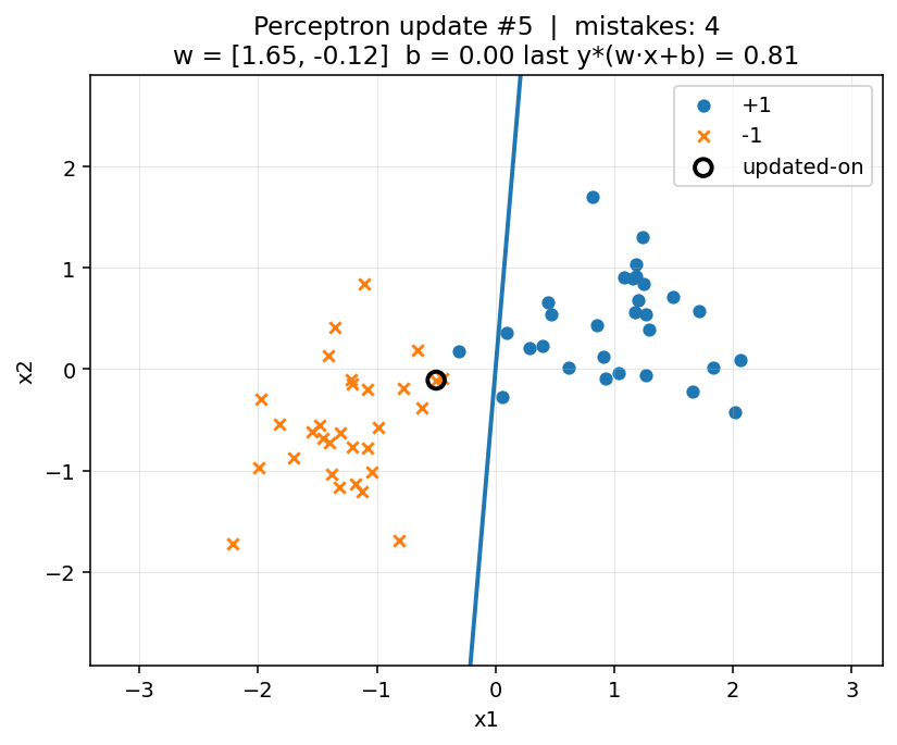
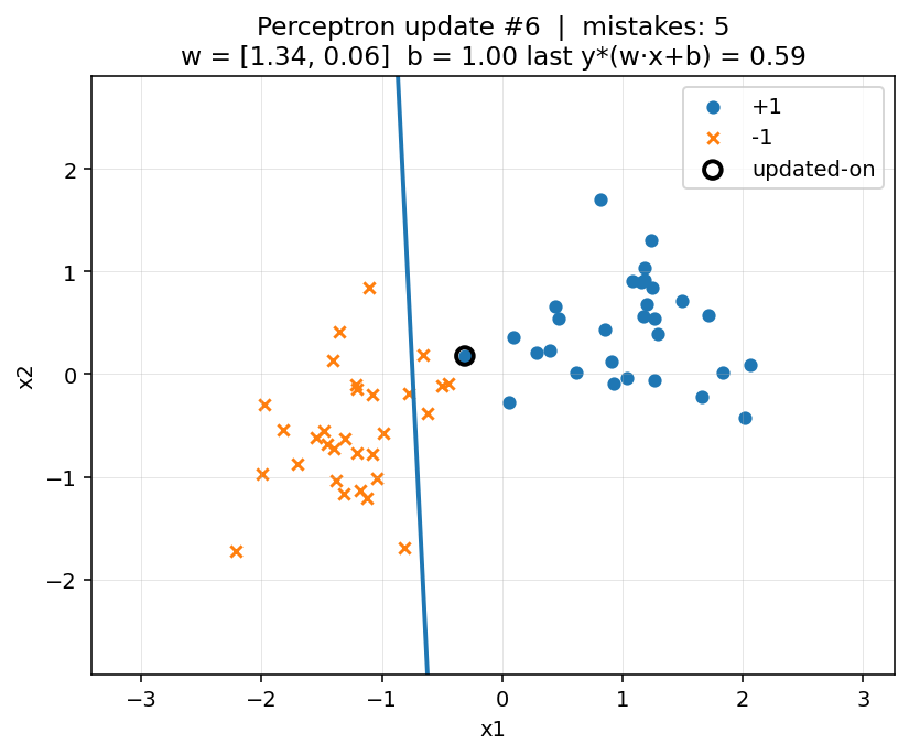
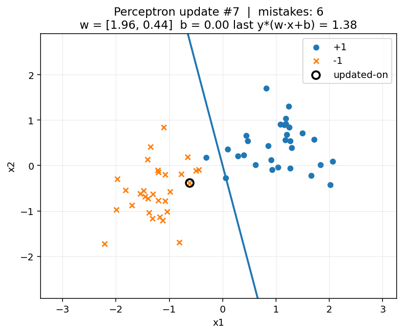
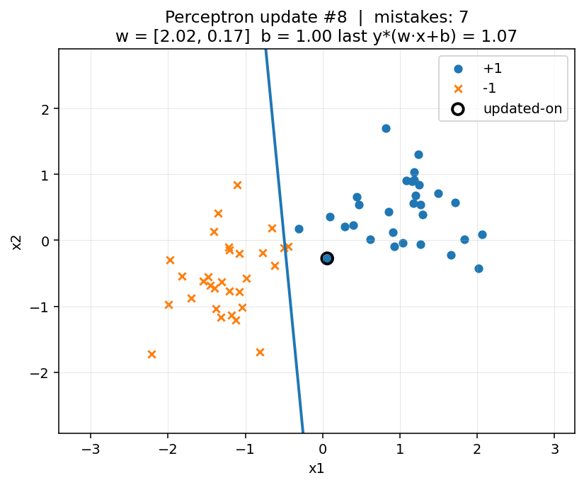
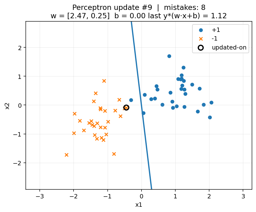
Perceptron learning rule (online)
For each example \((x^{(i)}, y^{(i)})\):
- Predict \(\hat y = \operatorname{sign}(w^\top x^{(i)} + b)\).
- If correct (i.e., \(y^{(i)}\hat y = +1\)), do nothing.
- If mistake (i.e., \(y^{(i)}\hat y = -1\)), update \[ w \leftarrow w + \eta\, y^{(i)} x^{(i)}, \qquad b \leftarrow b + \eta\, y^{(i)}. \]
\(\eta>0\) is the learning rate (a hyperparameter). With the bias trick: \(\tilde w \leftarrow \tilde w + \eta\, y^{(i)} \tilde x^{(i)}\).
Why the update makes sense
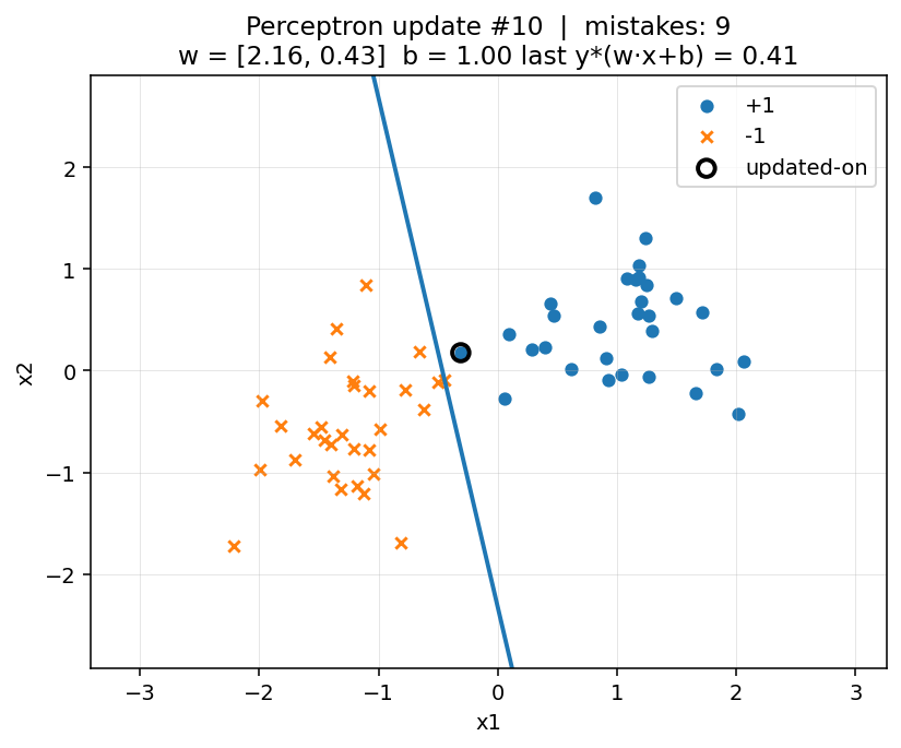
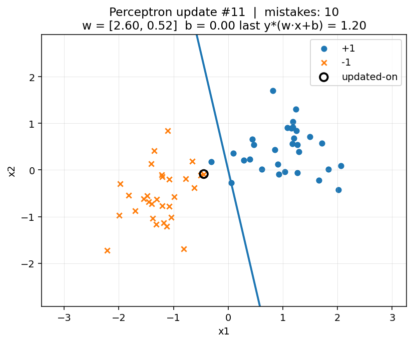
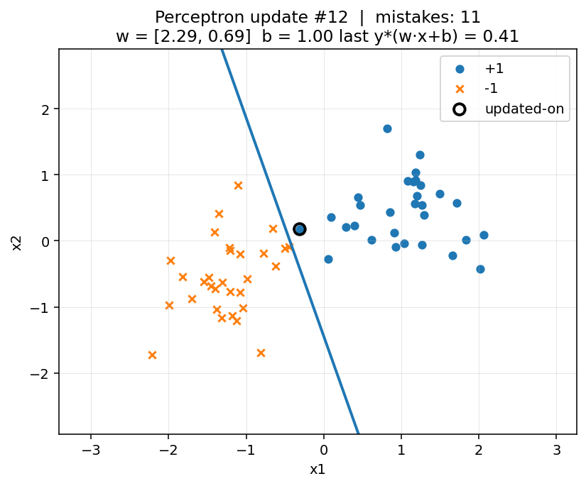
On a mistake, \(y^{(i)}(w^\top x^{(i)} + b) < 0\). The update adds a vector in the direction of \(y^{(i)} x^{(i)}\), increasing the signed margin \(y^{(i)}(w^\top x^{(i)} + b)\).
Geometrically: it nudges the decision boundary toward correctly placing the misclassified point on the right side.
Pseudocode
# initialize
w = 0; b = 0
for epoch in 1..T:
  shuffle(training_data)
  for (x, y) in training_data:
      if y * (w·x + b) ≤ 0:   # mistake
          w ← w + η * y * x
          b ← b + η * y
(Many implementations simply set \(\eta=1\) for separable problems; scaling of \(w\) does not change decisions.)
Convergence (when it works)
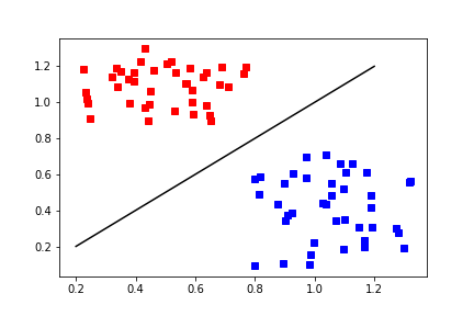
- If the data are linearly separable with margin \(\gamma>0\) and all \(\|x\|\le R\), the algorithm makes at most \(\mathcal O\big((R/\gamma)^2\big)\) mistakes and converges (Novikoff bound).
- Otherwise, it may cycle forever; in practice we cap epochs.
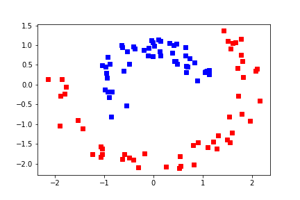
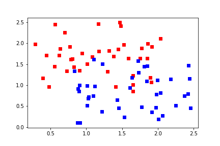
Linearly separable?
Separable (linear)
Not linearly separable
Real data are often almost separable with noise/outliers.
When it struggles
- Non-separable data (e.g., XOR) ⇒ no single hyperplane can separate.
- Zero margin / outliers ⇒ boundary hugs points ⇒ poor generalisation.
- Order sensitivity ⇒ shuffling typically helps.
Practical tips
- Standardise/normalise features; include an explicit bias or use the bias trick.
- Shuffle each epoch; limit epochs; consider early stopping on a validation set.
- Set \(\eta\) (e.g., 1.0) or use a small decay; for separable cases, \(\eta\) mainly affects speed.
Useful variants (still simple)
- Averaged perceptron: predict with the running average of weights; often generalises better.
- Perceptron with margin: only update if \(y(w^\top x + b) \le \delta\) for margin \(\delta>0\).
- Feature maps / kernels: map inputs so a hyperplane exists in feature space.
Perceptron Summary
- Perceptron is a simple online algorithm for linear decision boundaries.
- Converges on linearly separable data; otherwise use caps/variants.
- Forms a conceptual bridge to modern linear models and neural nets.
Summary
In this lecture, we covered the following key concepts in Machine Learning:
- Types of Problems: Classification, Regression, Clustering, and Dimensionality Reduction.
- Types of Learning: Supervised, Unsupervised, Semi-supervised, and Reinforcement Learning.
- Perceptron Algorithm: A foundational model for binary classification and its key features and limitations.
Machine Learning is a broad and evolving field that bridges data, algorithms, and real-world applications. Understanding these concepts forms a solid foundation for deeper exploration into modern ML techniques and applications.